Processing and integrating PBMC TEA-seq data#

This notebooks provides an example for TEA-seq data processing in Python.

TEA-seq is a method for trimodal single-cell profiling that allows to get gene expression, chromatin accessibility, and epitope information per cell. The method is described in Swanson et al., 2021.

The data used in this notebook is on peripheral blood mononuclear cells (PBMCs) and can be downloaded from GEO. We will use a single TEA-seq sample in this notebook — GSM5123951.

[1]:

# Change directory to the root folder of the repository
import os
os.chdir("../../")

Import libraries#

[2]:

import numpy as np
import pandas as pd
import scanpy as sc

[3]:

import muon as mu
import muon.atac as ac
import muon.prot as pt

[4]:

import matplotlib
from matplotlib import pyplot as plt
plt.rcParams['figure.dpi'] = 100

Prepare & load data#

We will use *_cellranger-arc_filtered_feature_bc_matrix.h5 and *_adt_counts.csv.gz files with counts. For chromatin accessibility, we’ll also use *_atac_filtered_fragments.tsv.gz files with fragments as well as metadata in *_atac_filtered_metadata.csv.gz.

For this notebook, we work with a single sample.

[5]:

# This is the directory where those files are downloaded to
data_dir = "data/teaseq"

[6]:

from glob import glob
for file in glob(f"{data_dir}/GSM5123951*"):
    print(file)

data/teaseq/GSM5123951_X066-MP0C1W3_leukopak_perm-cells_tea_200M_atac_filtered_metadata.csv.gz
data/teaseq/GSM5123951_X066-MP0C1W3_leukopak_perm-cells_tea_200M_atac_filtered_fragments.tsv.gz.tbi
data/teaseq/GSM5123951_X066-MP0C1W3_leukopak_perm-cells_tea_48M_adt_counts.csv.gz
data/teaseq/GSM5123951_X066-MP0C1W3_leukopak_perm-cells_tea_200M_atac_filtered_fragments.tsv.gz
data/teaseq/GSM5123951_X066-MP0C1W3_leukopak_perm-cells_tea_200M_cellranger-arc_filtered_feature_bc_matrix.h5

Construct simple metadata parsed from the filenames:

[7]:

meta = {}
for file in glob(f"{data_dir}/GSM5123951*"):
    tokens = os.path.basename(file).split("_")
    meta[
        tokens[0]       # GSM5123951
    ] = tokens[1][-2:]  # W3

meta

[7]:

{'GSM5123951': 'W3'}

First, we will load RNA+ATAC counts.

[8]:

get_h5_file = lambda root, s, w: f"{root}/{s}_X066-MP0C1{w}_leukopak_perm-cells_tea_200M_cellranger-arc_filtered_feature_bc_matrix.h5"

s, w = list(meta.items())[0]

mdata = mu.read_10x_h5(
    get_h5_file(data_dir, s, w)
)

mdata.obs["sample"] = s
mdata.obs["well"] = w

mdata.update()
mdata.var_names_make_unique()

/usr/local/bin/miniconda3/envs/issue57/lib/python3.8/site-packages/anndata/_core/anndata.py:1830: UserWarning: Variable names are not unique. To make them unique, call `.var_names_make_unique`.
  utils.warn_names_duplicates("var")

Added `interval` annotation for features from data/teaseq/GSM5123951_X066-MP0C1W3_leukopak_perm-cells_tea_200M_cellranger-arc_filtered_feature_bc_matrix.h5

/usr/local/bin/miniconda3/envs/issue57/lib/python3.8/site-packages/anndata/_core/anndata.py:1830: UserWarning: Variable names are not unique. To make them unique, call `.var_names_make_unique`.
  utils.warn_names_duplicates("var")
mudata/_core/mudata.py:437: UserWarning: var_names are not unique. To make them unique, call `.var_names_make_unique`.
  warnings.warn(
mudata/mudata/_core/mudata.py:437: UserWarning: var_names are not unique. To make them unique, call `.var_names_make_unique`.
  warnings.warn(

[9]:

mdata

[9]:

MuData object with n_obs × n_vars = 7966 × 138155
  obs:      'sample', 'well'
  var:      'gene_ids', 'feature_types', 'genome', 'interval'
  2 modalities
    rna:    7966 x 36601
      var:  'gene_ids', 'feature_types', 'genome', 'interval'
    atac:   7966 x 101554
      var:  'gene_ids', 'feature_types', 'genome', 'interval'

We can use rich representation to explore the structure of the object.

[10]:

mu.set_options(display_style="html", display_html_expand=0b000);

[11]:

mdata

[11]:

MuData object 7966 obs × 138155 var in 2 modalities

Metadata

.obs2 elements

sample	object	GSM5123951,GSM5123951,GSM5123951,GSM5123951,...
well	object	W3,W3,W3,W3,W3,W3,W3,W3,W3,W3,W3,W3,W3,W3,W3,W3,...

Embeddings & mappings

.obsm0 elements

No embeddings & mappings

Distances

.obsp0 elements

No distances

rna

7966 × 36601

AnnData object 7966 obs × 36601 var

Matrix

float32 scipy.sparse._csr.csr_matrix

Layers

.layers0 elements

No layers

Metadata

.obs0 elements

No metadata

Embeddings

.obsm0 elements

No embeddings

Distances

.obsp0 elements

No distances

Miscellaneous

.uns0 elements

No miscellaneous

atac

7966 × 101554

AnnData object 7966 obs × 101554 var

Matrix

float32 scipy.sparse._csr.csr_matrix

Layers

.layers0 elements

No layers

Metadata

.obs0 elements

No metadata

Embeddings

.obsm0 elements

No embeddings

Distances

.obsp0 elements

No distances

Miscellaneous

.uns0 elements

No miscellaneous

Then we will load protein counts.

[12]:

prot_counts = pd.read_csv(f"{data_dir}/{s}_X066-MP0C1{w}_leukopak_perm-cells_tea_48M_adt_counts.csv.gz")
prot_counts.set_index("cell_barcode", inplace=True)
prot_counts_total = prot_counts.total.values
del prot_counts["total"]

[13]:

prot_raw = mu.AnnData(X=prot_counts)
prot_raw.obs["total_counts"] = prot_counts_total

prot_raw.obs_names = prot_raw.obs_names + "-1"
prot_raw.var_names = "prot:" + prot_raw.var_names  # feature names will be unambiguous then (e.g. gene or protein)

/var/folders/xt/tvy3s7w17vn1b700k_351pz00000gp/T/ipykernel_62585/1322958841.py:1: FutureWarning: X.dtype being converted to np.float32 from int64. In the next version of anndata (0.9) conversion will not be automatic. Pass dtype explicitly to avoid this warning. Pass `AnnData(X, dtype=X.dtype, ...)` to get the future behavour.
  prot_raw = mu.AnnData(X=prot_counts)

[14]:

prot_raw

[14]:

AnnData object with n_obs × n_vars = 720873 × 46
    obs: 'total_counts'

[15]:

prot_raw.var_names.values

[15]:

array(['prot:CD10', 'prot:CD11b', 'prot:CD11c', 'prot:CD123',
       'prot:CD127', 'prot:CD14', 'prot:CD141', 'prot:CD16',
       'prot:CD172a', 'prot:CD185', 'prot:CD19', 'prot:CD192',
       'prot:CD197', 'prot:CD21', 'prot:CD24', 'prot:CD25', 'prot:CD269',
       'prot:CD27', 'prot:CD278', 'prot:CD279', 'prot:CD3', 'prot:CD304',
       'prot:CD319', 'prot:CD38', 'prot:CD39', 'prot:CD4', 'prot:CD40',
       'prot:CD45RA', 'prot:CD45RO', 'prot:CD56', 'prot:CD66b',
       'prot:CD71', 'prot:CD80', 'prot:CD86', 'prot:CD8a', 'prot:CD95',
       'prot:FceRI', 'prot:HLA-DR', 'prot:IgD',
       'prot:IgG1-K-Isotype-Control', 'prot:IgM', 'prot:KLRG1',
       'prot:TCR-Va24-Ja18', 'prot:TCR-Va7.2', 'prot:TCR-a/b',
       'prot:TCR-g/d'], dtype=object)

This is a 'raw' matrix, in which both cells and empty droplets are present. We will take advantage of this for denoising protein counts.

We can add a protein modality to our multimodal container. We will only add droplets with cells.

[16]:

mdata.mod["prot"] = prot_raw[mdata.obs_names].copy()
mdata.update()

[17]:

mdata

[17]:

MuData object 7966 obs × 138201 var in 3 modalities

Metadata

.obs3 elements

prot:total_counts	int64	863,957,1108,899,1155,835,820,643,822,776,406,...
sample	object	GSM5123951,GSM5123951,GSM5123951,GSM5123951,...
well	object	W3,W3,W3,W3,W3,W3,W3,W3,W3,W3,W3,W3,W3,W3,W3,W3,...

Embeddings & mappings

.obsm0 elements

No embeddings & mappings

Distances

.obsp0 elements

No distances

rna

7966 × 36601

AnnData object 7966 obs × 36601 var

Matrix

float32 scipy.sparse._csr.csr_matrix

Layers

.layers0 elements

No layers

Metadata

.obs0 elements

No metadata

Embeddings

.obsm0 elements

No embeddings

Distances

.obsp0 elements

No distances

Miscellaneous

.uns0 elements

No miscellaneous

atac

7966 × 101554

AnnData object 7966 obs × 101554 var

Matrix

float32 scipy.sparse._csr.csr_matrix

Layers

.layers0 elements

No layers

Metadata

.obs0 elements

No metadata

Embeddings

.obsm0 elements

No embeddings

Distances

.obsp0 elements

No distances

Miscellaneous

.uns0 elements

No miscellaneous

prot

7966 × 46

AnnData object 7966 obs × 46 var

Matrix

float32 numpy.ndarray

Layers

.layers0 elements

No layers

Metadata

.obs1 element

total_counts

int64

863,957,1108,899,1155,835,820,643,822,776,406,...

Embeddings

.obsm0 elements

No embeddings

Distances

.obsp0 elements

No distances

Miscellaneous

.uns0 elements

No miscellaneous

Processing individual modalities#

Protein modality (epitopes)#

[18]:

prot = mdata["prot"]

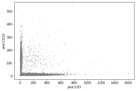
DSB normalisation#

This normalisation method developed for CITE-seq data uses background droplets defined by low RNA content in order to estimate background protein signal and remove it from the data. More details and its original implementation are available in the ``dsb` GitHub repository <https://github.com/niaid/dsb>`__.

Preserve original counts in a layer before the normalisation:

[19]:

prot.layers['counts'] = prot.X

Specify features corresponding to the isotype controls:

[20]:

isotypes = prot.var_names.values[["Isotype" in v for v in prot.var_names]]
print(isotypes)

['prot:IgG1-K-Isotype-Control']

Normalize counts with dsb:

[21]:

pt.pp.dsb(mdata, prot_raw, isotype_controls=isotypes, random_state=1)

muon/muon/_prot/preproc.py:109: UserWarning: empty_counts_range values are not provided, treating all the non-cells as empty droplets
  warn(

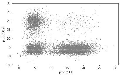
Plot values to visualise the effect of normalisation:

[22]:

sc.pl.scatter(mdata['prot'], x="prot:CD3", y="prot:CD19", layers='counts')
sc.pl.scatter(mdata['prot'], x="prot:CD3", y="prot:CD19")

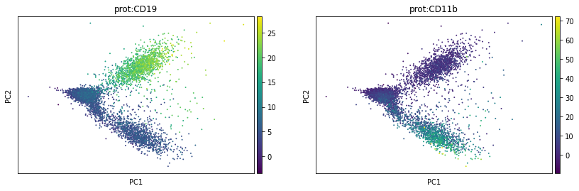
../../_images/trimodal_tea-seq_1-TEA-seq-PBMC_40_0.png

../../_images/trimodal_tea-seq_1-TEA-seq-PBMC_40_1.png

Downstream analysis#

We can run conventional methods like PCA on the normalised protein counts:

[23]:

sc.tl.pca(prot)

[24]:

sc.pl.pca(prot, color=['prot:CD19', 'prot:CD11b'])

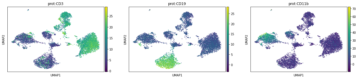
../../_images/trimodal_tea-seq_1-TEA-seq-PBMC_44_0.png

[25]:

sc.pp.neighbors(prot)
sc.tl.umap(prot, random_state=1)

[26]:

sc.pl.umap(prot, color=['prot:CD3', 'prot:CD19', 'prot:CD11b'])

../../_images/trimodal_tea-seq_1-TEA-seq-PBMC_46_0.png

RNA modality#

[27]:

rna = mdata.mod['rna']
rna

[27]:

AnnData object with n_obs × n_vars = 7966 × 36601
    var: 'gene_ids', 'feature_types', 'genome', 'interval'

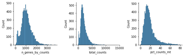
QC#

Perform some quality control. For now, we will filter out cells that do not pass QC from the whole dataset.

[28]:

rna.var['mt'] = rna.var_names.str.startswith('MT-')  # annotate the group of mitochondrial genes as 'mt'
sc.pp.calculate_qc_metrics(rna, qc_vars=['mt'], percent_top=None, log1p=False, inplace=True)

[29]:

mu.pl.histogram(rna, ['n_genes_by_counts', 'total_counts', 'pct_counts_mt'])

../../_images/trimodal_tea-seq_1-TEA-seq-PBMC_52_0.png

Filter genes which expression is not detected:

[30]:

mu.pp.filter_var(rna, 'n_cells_by_counts', lambda x: x >= 10)  # gene detected at least in 10 cells

Filter cells:

[31]:

mu.pp.filter_obs(rna, 'n_genes_by_counts', lambda x: (x >= 200) & (x < 2500))

mu.pp.filter_obs(rna, 'total_counts', lambda x: (x > 500) & (x < 5000))
mu.pp.filter_obs(rna, 'pct_counts_mt', lambda x: x < 30)

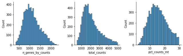
Let’s see how the data looks after filtering:

[32]:

mu.pl.histogram(rna, ['n_genes_by_counts', 'total_counts', 'pct_counts_mt'])

../../_images/trimodal_tea-seq_1-TEA-seq-PBMC_58_0.png

Normalisation#

We’ll normalise the data so that we get log-normalised counts to work with.

[33]:

sc.pp.normalize_total(rna, target_sum=1e4)

[34]:

sc.pp.log1p(rna)

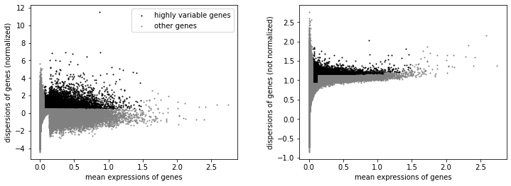
Feature selection#

We will label highly variable genes that we’ll use for downstream analysis.

[35]:

sc.pp.highly_variable_genes(rna, min_mean=0.02, max_mean=4, min_disp=0.5)

[36]:

sc.pl.highly_variable_genes(rna)

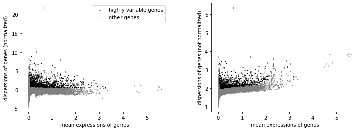
../../_images/trimodal_tea-seq_1-TEA-seq-PBMC_66_0.png

[37]:

np.sum(rna.var.highly_variable)

[37]:

Scaling#

We’ll save log-normalised counts in the "lognorm" layer:

[38]:

rna.layers["lognorm"] = rna.X.copy()

… and scale the log-normalised counts to zero mean and unit variance:

[39]:

sc.pp.scale(rna, max_value=10)

Downstream analysis#

Having filtered low-quality cells, normalised the counts matrix, and performed feature selection, we can already use this data for multimodal integration.

It is usually a good idea to study individual modalities first. Moreover, some multimodal methods can utilize principal components space or cell neighbourhood graphs from individual modalities.

Below we run PCA on the scaled matrix, compute cell neighbourhood graph, and perform clustering to define cell types.

PCA and neighbourhood graph#

[40]:

sc.tl.pca(rna, svd_solver='arpack')

To visualise the result, we will use some markers for (large-scale) cell populations we expect to see such as T cells and NK cells (CD2), B cells (CD79A), and KLF4 (monocytes).

[41]:

sc.pl.pca(rna, color=['CD2', 'CD3E', 'NKG7', 'KLF4', 'MS4A1', 'CD79A', 'IRF8'], layer="lognorm")

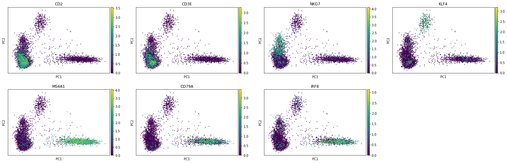
../../_images/trimodal_tea-seq_1-TEA-seq-PBMC_78_0.png

The first principal component (PC1) is separating T/NK (left), myeloid (middle), and B (right) cells while monocyte-related features seem to drive the second one. Also we see plasmocytoid dendritic cells (marked by IRF8) being close to B cells in the PC1/PC2 space.

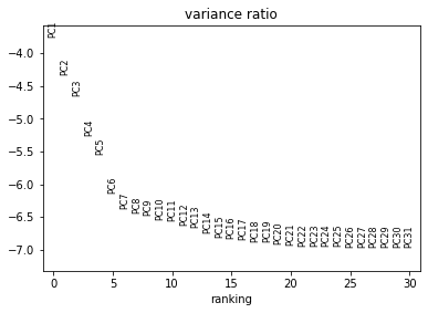
[42]:

sc.pl.pca_variance_ratio(rna, log=True)

../../_images/trimodal_tea-seq_1-TEA-seq-PBMC_80_0.png

Now we can compute a neighbourhood graph for cells:

[43]:

sc.pp.neighbors(rna, n_neighbors=10, n_pcs=20)

Non-linear dimensionality reduction and clustering#

With the neighbourhood graph computed, we can now perform clustering. We will use leiden clustering as an example.

[44]:

sc.tl.leiden(rna, resolution=.75)

To visualise the results, we’ll first generate a 2D latent space with cells that we can colour according to their cluster assignment.

[45]:

sc.tl.umap(rna, spread=1., min_dist=.5, random_state=11)

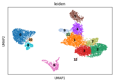
[46]:

sc.pl.umap(rna, color="leiden", legend_loc="on data")

../../_images/trimodal_tea-seq_1-TEA-seq-PBMC_88_0.png

Plotting across modalities#

With mu.pl.embedding interface we can display an embedding from an individual modality (e.g. 'rna') and colour cells by a feature (variable) from another modality.

While variables names should be unique across all modalities, all individual modalities as well as the mdata object itself can have e.g. UMAP basis computed. To point to a basis from a specific modality, use mod:basis syntax, e.g. with "rna:X_umap" in the example below mdata.mod['rna'].obsm["X_umap"] basis is going to be used.

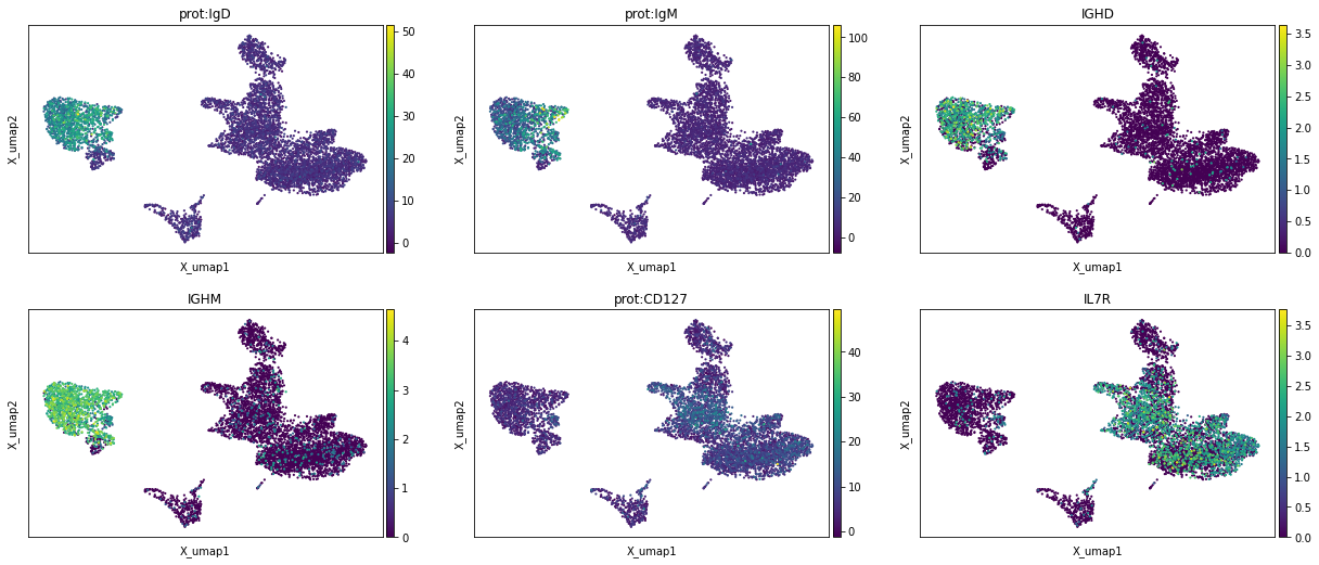
[48]:

mu.pl.embedding(mdata, basis="rna:X_umap", color=["prot:IgD", "prot:IgM", "IGHD", "IGHM", "prot:CD127", "IL7R"], layer={"rna": "lognorm"}, ncols=3)

../../_images/trimodal_tea-seq_1-TEA-seq-PBMC_91_0.png

ATAC modality#

[49]:

atac = mdata['atac']
atac

[49]:

AnnData object with n_obs × n_vars = 7966 × 101554
    var: 'gene_ids', 'feature_types', 'genome', 'interval'

Locate the fragments file (use tabix -p bed to generate an index file for it):

[50]:

ac.tl.locate_fragments(atac, f"{data_dir}/{s}_X066-MP0C1{w}_leukopak_perm-cells_tea_200M_atac_filtered_fragments.tsv.gz")

Adding metadata to the ATAC modality:

[51]:

metadata = pd.read_csv(f"{data_dir}/{s}_X066-MP0C1{w}_leukopak_perm-cells_tea_200M_atac_filtered_metadata.csv.gz")
pd.set_option('display.max_columns', 500)
metadata.head()

[51]:

	original_barcodes	n_fragments	n_duplicate	n_mito	n_unique	altius_count	altius_frac	gene_bodies_count	gene_bodies_frac	peaks_count	peaks_frac	tss_count	tss_frac	barcodes	cell_name	well_id	chip_id	batch_id	pbmc_sample_id	DoubletScore	DoubletEnrichment	TSSEnrichment
0	GTGTGAGCATGCTATG-1	38760	17870	2	17316	13692	0.790714	11785	0.680584	10043	0.579984	5100	0.294525	69c6c7c43ef411ebb8b442010a19c80f	unblacked_accurate_myotis	X066-AP0C1W3	X066-AP0C1	X066	X066-Well3	0.000000	0.257143	8.046
1	TCACCGGCACAGAACG-1	12820	7294	12	4291	3751	0.874155	3128	0.728968	3159	0.736192	2194	0.511303	69c7d3ee3ef411ebb8b442010a19c80f	fabulous_panphobic_tahr	X066-AP0C1W3	X066-AP0C1	X066	X066-Well3	0.000000	0.114286	8.997
2	AAAGGACGTACAATGT-1	16117	9524	0	4989	4561	0.914211	3602	0.721988	3863	0.774303	2828	0.566847	69be295c3ef411ebb8b442010a19c80f	tricky_anaemic_mayfly	X066-AP0C1W3	X066-AP0C1	X066	X066-Well3	0.000000	0.085714	11.081
3	CAGCCTAAGACAACAG-1	44967	24156	0	17456	15918	0.911893	12033	0.689333	13724	0.786205	7241	0.414814	69c161123ef411ebb8b442010a19c80f	agonizing_haughty_collie	X066-AP0C1W3	X066-AP0C1	X066	X066-Well3	2.351825	1.828571	12.804
4	ACTCGCTTCCAGGAAA-1	16526	8896	0	6227	5584	0.896740	4286	0.688293	4747	0.762325	2658	0.426851	69bf6b003ef411ebb8b442010a19c80f	exorcistic_harmonic_bushbaby	X066-AP0C1W3	X066-AP0C1	X066	X066-Well3	0.000000	1.400000	21.016

[52]:

atac.obs = atac.obs.join(metadata.set_index("original_barcodes"))

Please note this metadata is available for the filtered (after QC) ATAC data so this modality can be just filtered using these cells.

For demonstration purposes we will still go through processing steps before removing barcodes that were filtered out.

QC#

Perform some quality control filtering out cells with too few peaks and peaks detected in too few cells. For now, we will filter out cells that do not pass QC.

[53]:

sc.pp.calculate_qc_metrics(atac, percent_top=None, log1p=False, inplace=True)

[54]:

mu.pl.histogram(atac, ['total_counts', 'n_genes_by_counts'])

../../_images/trimodal_tea-seq_1-TEA-seq-PBMC_103_0.png

Filter peaks which expression is not detected:

[55]:

mu.pp.filter_var(atac, 'n_cells_by_counts', lambda x: x >= 5)  # a peak is detected in 5 cells or more

Filter cells:

[56]:

mu.pp.filter_obs(atac, 'total_counts', lambda x: (x >= 1000) & (x <= 30000))

mu.pp.filter_obs(atac, 'n_genes_by_counts', lambda x: (x >= 500) & (x <= 10000))  # number of peaks per cell

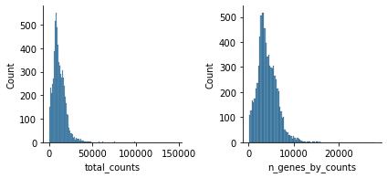
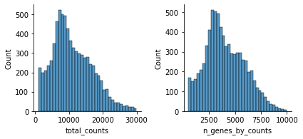
Let’s see how the data looks after filtering:

[57]:

mu.pl.histogram(atac, ['total_counts', 'n_genes_by_counts'])

../../_images/trimodal_tea-seq_1-TEA-seq-PBMC_109_0.png

There are a few expectations about how ATAC-seq data looks like as noted in the hitchhiker’s guide to ATAC-seq data analysis for instance.

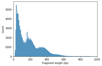
Nucleosome signal#

Fragment size distribution typically reflects nucleosome binding pattern showing enrichment around values corresponding to fragments bound to a single nucleosome (between 147 bp and 294 bp) as well as nucleosome-free fragments (shorter than 147 bp).

[58]:

ac.pl.fragment_histogram(atac, region='chr1:1-2000000', barcodes="barcodes")

Fetching Regions...: 100%|███████████████████████████████████████████████████████████████████████████████████████████████████████████████████████████████████████████████████████████████████████████████████| 1/1 [00:00<00:00,  1.19it/s]

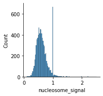
../../_images/trimodal_tea-seq_1-TEA-seq-PBMC_113_1.png

The ratio of mono-nucleosome cut fragments to nucleosome-free fragments can be called nucleosome signal, and it can be estimated using a subset of fragments.

[59]:

ac.tl.nucleosome_signal(atac, n=1e6, barcodes="barcodes")

Reading Fragments: 100%|█████████████████████████████████████████████████████████████████████████████████████████████████████████████████████████████████████████████████████████████████████| 1000000/1000000 [00:06<00:00, 149011.41it/s]

[60]:

mu.pl.histogram(atac, "nucleosome_signal", kde=False)

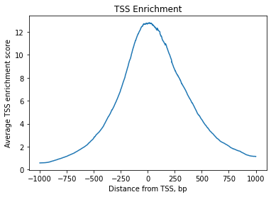
../../_images/trimodal_tea-seq_1-TEA-seq-PBMC_116_0.png

TSS enrichment#

We can expect chromatin accessibility enriched around transcription start sites (TSS) compared to accessibility of flanking regions. Thus this measure averaged across multiple genes can serve as one more quality control metric.

The positions of transcription start sites can be obtained from the interval field of the gene annotation in the rna modality:

[61]:

ac.tl.get_gene_annotation_from_rna(mdata['rna']).head(3)  # accepts MuData with 'rna' modality or mdata['rna'] AnnData directly

[61]:

	Chromosome	Start	End	gene_id	gene_name
AL627309.5	chr1	149706	173862	ENSG00000241860	AL627309.5
LINC01409	chr1	778757	803934	ENSG00000237491	LINC01409
LINC01128	chr1	827597	860227	ENSG00000228794	LINC01128

TSS enrichment function will return an AnnData object with cells x bases dimensions where bases correspond to positions around TSS and are defined by extend_upstream and extend_downstream parameters, each of them being 1000 bp by default. It will also record tss_score in the original object.

[62]:

tss = ac.tl.tss_enrichment(mdata, n_tss=1000, barcodes="barcodes")  # by default, features=ac.tl.get_gene_annotation_from_rna(mdata)

Fetching Regions...: 100%|█████████████████████████████████████████████████████████████████████████████████████████████████████████████████████████████████████████████████████████████████████████████| 1000/1000 [00:16<00:00, 61.24it/s]

[63]:

tss

[63]:

AnnData object with n_obs × n_vars = 7639 × 2001
    obs: 'n_fragments', 'n_duplicate', 'n_mito', 'n_unique', 'altius_count', 'altius_frac', 'gene_bodies_count', 'gene_bodies_frac', 'peaks_count', 'peaks_frac', 'tss_count', 'tss_frac', 'barcodes', 'cell_name', 'well_id', 'chip_id', 'batch_id', 'pbmc_sample_id', 'DoubletScore', 'DoubletEnrichment', 'TSSEnrichment', 'n_genes_by_counts', 'total_counts', 'nucleosome_signal', 'tss_score'
    var: 'TSS_position'

[64]:

ac.pl.tss_enrichment(tss)

../../_images/trimodal_tea-seq_1-TEA-seq-PBMC_124_0.png

Now we’ll remove the barcodes that were filtered out as indicated in the provided metadata.

[65]:

# To avoid issues with nan being converted to 'nan' when the column is categorical,
# we explicitely convert it to str
mu.pp.filter_obs(atac, atac.obs.barcodes.astype(str) != 'nan')

Normalisation#

[66]:

# Save original counts
atac.layers["counts"] = atac.X

There can be multiple options for ATAC-seq data normalisation such as LSI that uses TF-IDF transformation.

Here we will use the same log-normalisation and PCA that we are used to from scRNA-seq analysis.

[67]:

sc.pp.normalize_per_cell(atac, counts_per_cell_after=1e4)
sc.pp.log1p(atac)

Feature selection#

We will label highly variable peaks that we’ll use for downstream analysis.

[68]:

sc.pp.highly_variable_genes(atac, min_mean=0.05, max_mean=1.5, min_disp=.5)

[69]:

sc.pl.highly_variable_genes(atac)

../../_images/trimodal_tea-seq_1-TEA-seq-PBMC_135_0.png

[70]:

np.sum(atac.var.highly_variable)

[70]:

Scaling#

We’ll save log-transformed counts in the "lognorm" layer:

[71]:

atac.layers["lognorm"] = atac.X.copy()

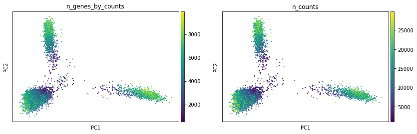
Downstream analysis#

PCA#

For this notebook, we are using PCA on the log-normalised counts in atac.X as described above.

[72]:

sc.pp.scale(atac)
sc.tl.pca(atac)

We can only colour our plots by cut counts in individual peaks with scanpy:

[73]:

sc.pl.pca(atac, color=["n_genes_by_counts", "n_counts"], layer="lognorm")

../../_images/trimodal_tea-seq_1-TEA-seq-PBMC_145_0.png

Now we will compute a neighbourhood graph for cells that we’ll use for clustering later on.

[74]:

sc.pp.neighbors(atac, n_neighbors=10, n_pcs=30)

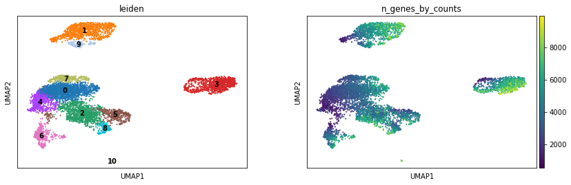
Non-linear dimensionality reduction and clustering#

To stay comparable to the gene expression notebook, we will use leiden to cluster cells.

[75]:

sc.tl.leiden(atac, resolution=.5)

We’ll use UMAP latent space for visualisation below.

[76]:

sc.tl.umap(atac, spread=1.5, min_dist=.5, random_state=30)

[77]:

sc.pl.umap(atac, color=["leiden", "n_genes_by_counts"], legend_loc="on data")

../../_images/trimodal_tea-seq_1-TEA-seq-PBMC_153_0.png

Multi-omics analyses#

For the downstream multimodal analysis, we will use only cells passing QC steps in each of the modality. Since cells were filtered out in each modality above, we can just take their intersection:

[78]:

mu.pp.intersect_obs(mdata)

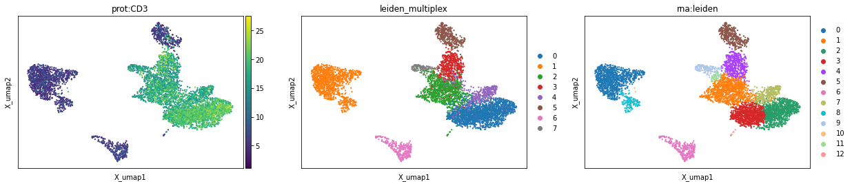
Multiplex clustering#

We can run clustering based on neighbours information from each modality taking advantage of multiplex versions of algorithms such as leiden or louvain.

[79]:

mdata.uns = dict()

[80]:

mu.tl.leiden(mdata, resolution=[1., 1., 1.], random_state=1, key_added="leiden_multiplex")

[85]:

mu.pl.embedding(mdata, basis="rna:X_umap", color=["prot:CD3", "leiden_multiplex", "rna:leiden"])

../../_images/trimodal_tea-seq_1-TEA-seq-PBMC_161_0.png

Multi-omics factor analysis#

To generate an interpretable latent space for all three modalities, we will now run multi-omic factor analysis — a group factor analysis method that will allow us to learn an interpretable latent space jointly on both modalities. Intuitively, it can be viewed as a generalisation of PCA for multi-omics data. More information about this method can be found on the MOFA website.

[86]:

prot.var["highly_variable"] = True
mdata.update()

[88]:

mu.tl.mofa(mdata, outfile="models/pbmc_w3_teaseq.hdf5")


        #########################################################
        ###           __  __  ____  ______                    ###
        ###          |  \/  |/ __ \|  ____/\    _             ###
        ###          | \  / | |  | | |__ /  \ _| |_           ###
        ###          | |\/| | |  | |  __/ /\ \_   _|          ###
        ###          | |  | | |__| | | / ____ \|_|            ###
        ###          |_|  |_|\____/|_|/_/    \_\              ###
        ###                                                   ###
        #########################################################



Loaded view='rna' group='group1' with N=5805 samples and D=2910 features...
Loaded view='atac' group='group1' with N=5805 samples and D=10867 features...
Loaded view='prot' group='group1' with N=5805 samples and D=46 features...


Model options:
- Automatic Relevance Determination prior on the factors: True
- Automatic Relevance Determination prior on the weights: True
- Spike-and-slab prior on the factors: False
- Spike-and-slab prior on the weights: True
Likelihoods:
- View 0 (rna): gaussian
- View 1 (atac): gaussian
- View 2 (prot): gaussian




######################################
## Training the model with seed 1 ##
######################################



Converged!



#######################
## Training finished ##
#######################


Warning: Output file models/pbmc_w3_teaseq.hdf5 already exists, it will be replaced
Saving model in models/pbmc_w3_teaseq.hdf5...
Saved MOFA embeddings in .obsm['X_mofa'] slot and their loadings in .varm['LFs'].

This adds X_mofa embeddings to the .obsm slot of the MuData object itself. The weights for the latent factors are stored in .varm["LFs"].

[89]:

mu.pl.mofa(mdata, color=['prot:CD3', 'prot:CD14'])

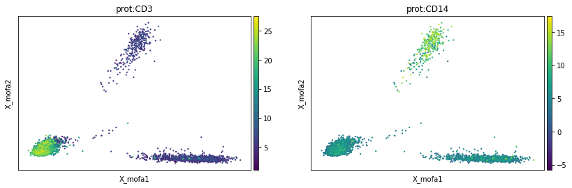
../../_images/trimodal_tea-seq_1-TEA-seq-PBMC_167_0.png

MOFA factors can be used to define cell neighbourhood graphs, which are thus based on all the modalities, as well as for subsequent non-linear latent space construction such as UMAP and clustering.

[90]:

sc.pp.neighbors(mdata, use_rep="X_mofa", key_added='mofa')
sc.tl.umap(mdata, min_dist=.2, random_state=1, neighbors_key='mofa')

[130]:

sc.tl.leiden(mdata, resolution=.3, neighbors_key='mofa', key_added='leiden_mofa')

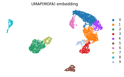
[131]:

mu.pl.umap(mdata, color=['leiden_mofa'], frameon=False, title="UMAP(MOFA) embedding")

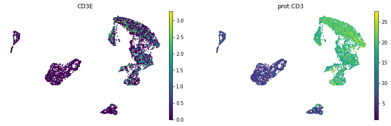
../../_images/trimodal_tea-seq_1-TEA-seq-PBMC_171_0.png

[93]:

mu.pl.umap(mdata, color=['CD3E', 'prot:CD3'], layer={"rna": "lognorm"}, frameon=False, cmap='viridis')

../../_images/trimodal_tea-seq_1-TEA-seq-PBMC_172_0.png

[95]:

mdata.obsm["X_mofa_umap"] = mdata.obsm["X_umap"].copy()

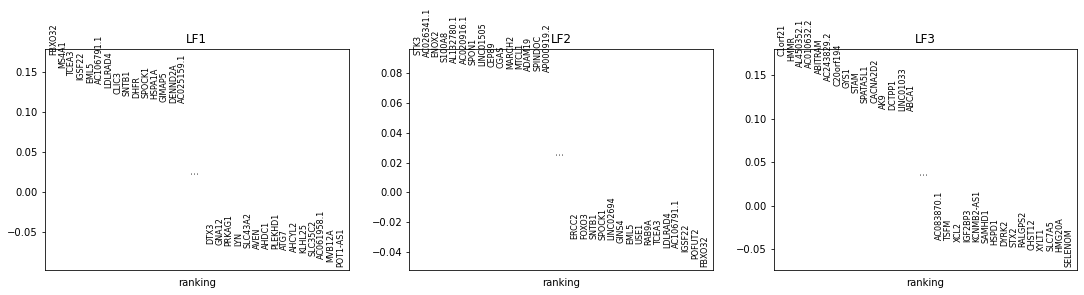
Interpreting the model#

We can describe factors by the top features, which they are defined by.

[96]:

mu.pl.mofa_loadings(mdata)

../../_images/trimodal_tea-seq_1-TEA-seq-PBMC_176_0.png

../../_images/trimodal_tea-seq_1-TEA-seq-PBMC_176_1.png

../../_images/trimodal_tea-seq_1-TEA-seq-PBMC_176_2.png

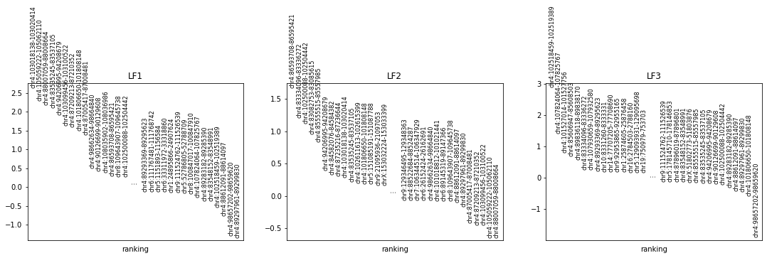
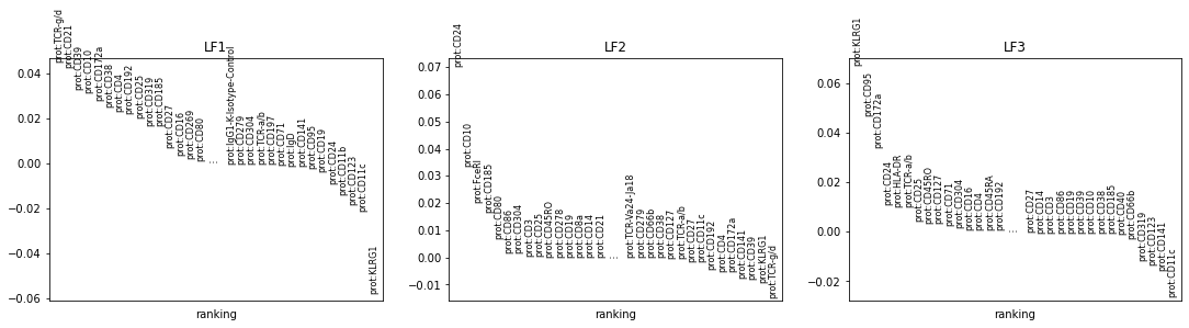
More detailed analysis of the MOFA model can be done with mofax, which is available here, using the model file saved during the training above.

Weighted nearest neighbours#

Another way to leverage multimodal information is with the weighted nearest neighbours (WNN) method, which constructs a multimodal cell neighbourhood graph based on cell neighbourhood graphs of individual modalities. muon implements WNN as it is described in `Hao et al., 2020 <>`__ with the generalisation to an arbitrary number of modalities proposed in Swanson et al., 2021.

For this to work, we’ll have to re-calculate neighbourhood in each modality because we have filtered out cells after that had been done above. That usually leads to having cells with no neighbours, and muon will be explicit about it and will return an error.

[97]:

for m in mdata.mod.keys():
    sc.pp.neighbors(mdata[m])

[98]:

mu.pp.neighbors(mdata, key_added='wnn')

Again, we can use the defined cell neighbours to perform clustering or non-linear dimensionality reduction.

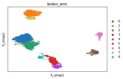
[145]:

sc.tl.leiden(mdata, resolution=.55, neighbors_key='wnn', key_added='leiden_wnn')

[148]:

mu.tl.umap(mdata, random_state=10, neighbors_key='wnn')

[149]:

mu.pl.umap(mdata, color="leiden_wnn")

../../_images/trimodal_tea-seq_1-TEA-seq-PBMC_186_0.png

[150]:

mdata.obsm["X_wnn_umap"] = mdata.obsm["X_umap"].copy()

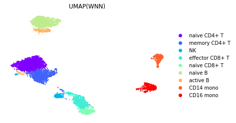
Cell types annotation#

We can use the results of any multiple multimodal analyses — or multiple ones — to define cell types. Alternatively, cell types can be defined using a single modality, e.g. 'prot', and the cell types labels robustness can then be checked with multimodal embeddings.

[151]:

mu.pl.embedding(mdata, basis="X_wnn_umap", color=list(map(
    lambda x: "prot:" + x,
    [
        "CD4", "CD45RA", "CD45RO",  # CD4 T cells
        "CD8a",                     # CD8 T cells
        "KLRG1",                    # NK cells
        "CD14", "CD16",             # monocytes
        "CD19", "CD21", "IgD",      # B cells
    ]
)))

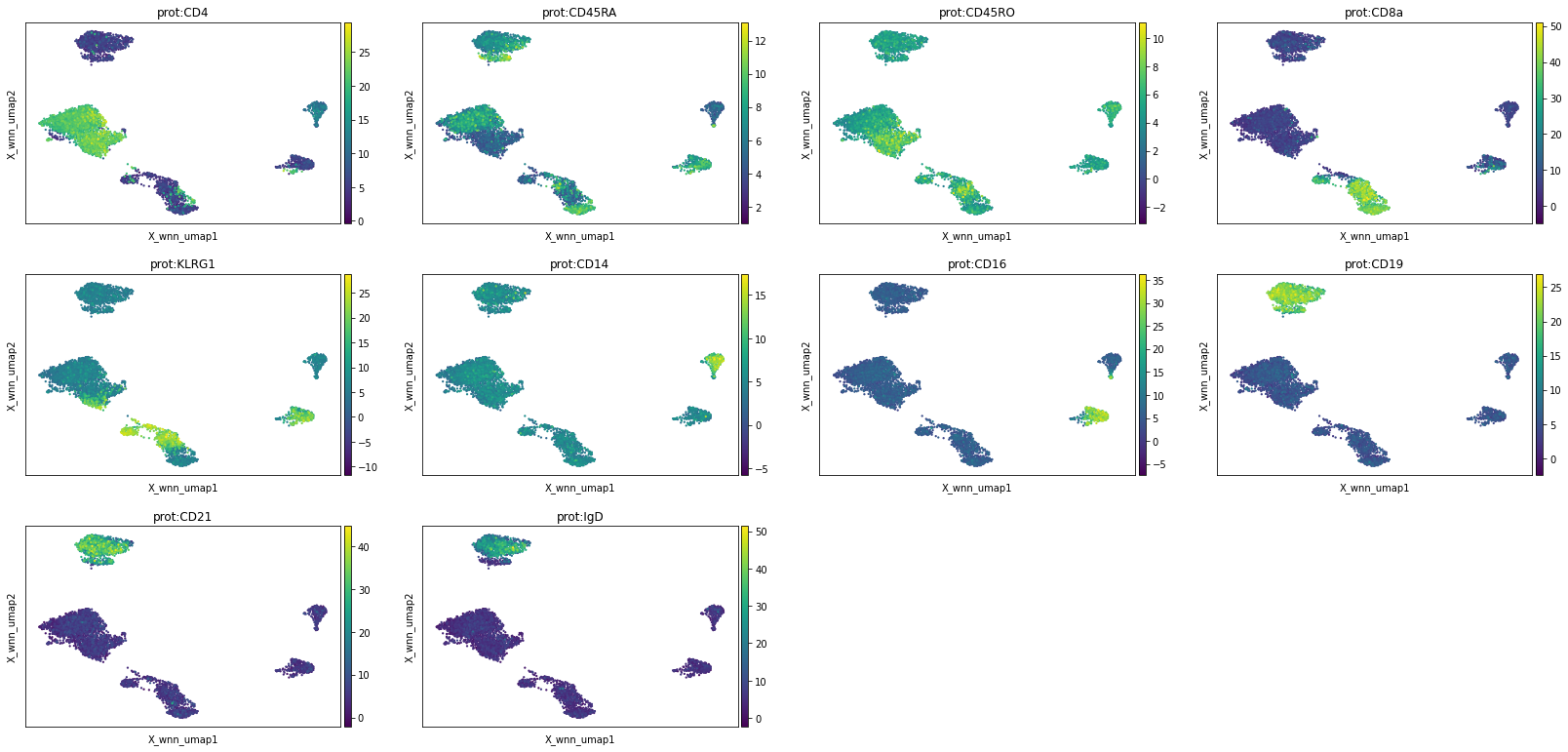
../../_images/trimodal_tea-seq_1-TEA-seq-PBMC_190_0.png

Label clusters according to the markers:

[155]:

new_cluster_names = {
    "0": "naïve CD4+ T", "1": "naïve B", "2": "memory CD4+ T",
    "4": "naïve CD8+ T", "3": "effector CD8+ T", "5": "CD16 mono",
    "6": "CD14 mono", "7": "active B", "8": "NK",
}

mdata.obs['celltype'] = mdata.obs.leiden_wnn.astype("str").values
mdata.obs.celltype = mdata.obs.celltype.astype("category")
mdata.obs.celltype = mdata.obs.celltype.cat.rename_categories(new_cluster_names)

[156]:

mdata.obs.celltype.cat.reorder_categories([
    'naïve CD4+ T', 'memory CD4+ T', 'NK', 'effector CD8+ T', 'naïve CD8+ T',
    'naïve B', 'active B',
    'CD14 mono', 'CD16 mono',
], inplace=True)

Add colours:

[157]:

cmap = plt.get_cmap('rainbow')
colors = cmap(np.linspace(0, 1, len(mdata.obs.celltype.cat.categories)))

mdata.uns["celltype_colors"] = list(map(matplotlib.colors.to_hex, colors))

[158]:

mu.pl.umap(mdata, color="celltype", frameon=False, title="UMAP(WNN)")

../../_images/trimodal_tea-seq_1-TEA-seq-PBMC_196_0.png

Saving multimodal data on disk#

[159]:

mdata.update()
mdata

[159]:

MuData object 5805 obs × 113187 var in 3 modalities

Metadata

.obs42 elements

rna:n_genes_by_counts	int32	1375,957,1052,1253,783,681,922,828,1083,1161,998,...
rna:total_counts	float32	2509.00,1405.00,1777.00,2399.00,1501.00,1018.00,...
rna:total_counts_mt	float32	200.00,119.00,298.00,277.00,448.00,144.00,411.00,...
rna:pct_counts_mt	float32	7.97,8.47,16.77,11.55,29.85,14.15,24.49,27.18,...
rna:leiden	object	2,2,7,0,8,3,8,3,5,1,0,2,2,2,1,2,6,0,3,0,0,4,4,1,1,...
atac:n_fragments	float64	13705.00,11567.00,25610.00,30969.00,16007.00,...
atac:n_duplicate	float64	8269.00,6897.00,15043.00,17513.00,8686.00,6703.00,...
atac:n_mito	float64	50.00,0.00,0.00,128.00,899.00,4.00,3.00,0.00,0.00,...
atac:n_unique	float64	4163.00,3516.00,8395.00,10883.00,4839.00,3152.00,...
atac:altius_count	float64	3777.00,3145.00,7613.00,9992.00,4314.00,2806.00,...
atac:altius_frac	float64	0.91,0.89,0.91,0.92,0.89,0.89,0.90,0.89,0.89,0.91,...
atac:gene_bodies_count	float64	3070.00,2545.00,6168.00,7951.00,3514.00,2263.00,...
atac:gene_bodies_frac	float64	0.74,0.72,0.73,0.73,0.73,0.72,0.71,0.72,0.74,0.74,...
atac:peaks_count	float64	3245.00,2648.00,6466.00,8669.00,3617.00,2408.00,...
atac:peaks_frac	float64	0.78,0.75,0.77,0.80,0.75,0.76,0.77,0.74,0.74,0.76,...
atac:tss_count	float64	2422.00,2053.00,5054.00,6165.00,2644.00,1812.00,...
atac:tss_frac	float64	0.58,0.58,0.60,0.57,0.55,0.57,0.54,0.57,0.59,0.57,...
atac:barcodes	object	69be0ea43ef411ebb8b442010a19c80f,...
atac:cell_name	object	viceregal_unconstant_hornet,...
atac:well_id	object	X066-AP0C1W3,X066-AP0C1W3,X066-AP0C1W3,...
atac:chip_id	object	X066-AP0C1,X066-AP0C1,X066-AP0C1,X066-AP0C1,...
atac:batch_id	object	X066,X066,X066,X066,X066,X066,X066,X066,X066,X066,...
atac:pbmc_sample_id	object	X066-Well3,X066-Well3,X066-Well3,X066-Well3,...
atac:DoubletScore	float64	0.00,0.00,0.00,0.00,0.00,11.71,0.00,0.83,0.00,...
atac:DoubletEnrichment	float64	0.37,1.23,1.26,0.69,0.89,2.46,0.34,1.69,1.00,0.74,...
atac:TSSEnrichment	float64	17.69,18.75,21.54,21.58,15.49,23.57,19.00,18.32,...
atac:n_genes_by_counts	int32	2846,2366,4987,6409,3105,2126,3849,2472,3107,4512,...
atac:total_counts	float32	7103.00,5916.00,14559.00,19267.00,8280.00,5259.00,...
atac:nucleosome_signal	float64	0.67,0.77,0.69,0.42,0.54,0.69,0.53,0.52,0.41,0.69,...
atac:tss_score	float64	9.91,5.17,6.09,4.33,6.03,10.30,5.83,3.20,14.67,...
atac:n_counts	float32	7102.00,5915.00,14559.00,19266.00,8280.00,5259.00,...
atac:leiden	object	0,0,7,1,9,4,9,0,6,2,1,0,0,0,2,0,3,1,0,1,1,5,2,2,4,...
prot:total_counts	int64	863,957,899,835,820,643,822,776,406,923,909,1320,...
sample	object	GSM5123951,GSM5123951,GSM5123951,GSM5123951,...
well	object	W3,W3,W3,W3,W3,W3,W3,W3,W3,W3,W3,W3,W3,W3,W3,W3,...
leiden_multiplex	object	0,0,4,1,1,0,1,0,5,3,1,0,0,0,2,0,6,1,0,1,1,3,4,2,2,...
leiden_mofa	category	0,0,6,2,7,0,7,0,5,3,2,4,0,0,1,4,8,7,0,7,2,3,3,1,1,...
rna:mod_weight	float64	0.33,0.30,0.34,0.30,0.30,0.33,0.21,0.32,0.33,0.31,...
atac:mod_weight	float64	0.33,0.30,0.33,0.30,0.26,0.35,0.29,0.33,0.34,0.31,...
prot:mod_weight	float64	0.35,0.40,0.33,0.40,0.45,0.33,0.50,0.36,0.33,0.39,...
leiden_wnn	category	0,0,4,1,7,0,7,0,5,3,1,0,0,0,2,0,6,1,0,1,1,3,3,2,2,...
celltype	category	naïve CD4+ T,naïve CD4+ T,naïve CD8+ T,naïve B,...

Embeddings & mappings

.obsm4 elements

X_mofa	float64	numpy.ndarray	10 dims
X_umap	float32	numpy.ndarray	2 dims
X_mofa_umap	float32	numpy.ndarray	2 dims
X_wnn_umap	float32	numpy.ndarray	2 dims

Distances

.obsp4 elements

mofa_distances	float64	scipy.sparse._csr.csr_matrix
mofa_connectivities	float32	scipy.sparse._csr.csr_matrix
wnn_distances	float32	scipy.sparse._csr.csr_matrix
wnn_connectivities	float32	scipy.sparse._csr.csr_matrix

Miscellaneous

.uns7 elements

leiden	dict	1 element	params: resolution,random_state,n_iterations
mofa	dict	3 elements	connectivities_key,distances_key,params
umap	dict	1 element	params: a,b,random_state
leiden_mofa_colors	list	11 elements	#1f77b4,#ff7f0e,#279e68,#d62728,#aa40fc,#8c564b,...
wnn	dict	3 elements	connectivities_key,distances_key,params
leiden_wnn_colors	list	11 elements	#1f77b4,#ff7f0e,#279e68,#d62728,#aa40fc,#8c564b,...
celltype_colors	list	9 elements	#8000ff,#4062fa,#00b5eb,#40ecd4,#80ffb4,#c0eb8d,...

rna

5805 × 16381

AnnData object 5805 obs × 16381 var

Matrix

float32 numpy.ndarray

Layers

.layers1 element

lognorm

float32

scipy.sparse._csr.csr_matrix

Metadata

.obs5 elements

n_genes_by_counts	int32	1375,957,1052,1253,783,681,922,828,1083,1161,998,...
total_counts	float32	2509.00,1405.00,1777.00,2399.00,1501.00,1018.00,...
total_counts_mt	float32	200.00,119.00,298.00,277.00,448.00,144.00,411.00,...
pct_counts_mt	float32	7.97,8.47,16.77,11.55,29.85,14.15,24.49,27.18,...
leiden	category	2,2,7,0,8,3,8,3,5,1,0,2,2,2,1,2,6,0,3,0,0,4,4,1,1,...

Embeddings

.obsm2 elements

X_pca	float32	numpy.ndarray	50 dims
X_umap	float32	numpy.ndarray	2 dims

Distances

.obsp2 elements

distances	float64	scipy.sparse._csr.csr_matrix
connectivities	float32	scipy.sparse._csr.csr_matrix

Miscellaneous

.uns7 elements

log1p	dict	1 element	base: None
hvg	dict	1 element	flavor: seurat
pca	dict	3 elements	params,variance,variance_ratio
neighbors	anndata.compat._overloaded_dict.OverloadedDict	3 elements	connectivities_key,distances_key,params
leiden	dict	1 element	params: resolution,random_state,n_iterations
umap	dict	1 element	params: a,b,random_state
leiden_colors	list	13 elements	#1f77b4,#ff7f0e,#279e68,#d62728,#aa40fc,#8c564b,...

atac

5805 × 96760

AnnData object 5805 obs × 96760 var

Matrix

float32 numpy.ndarray

Layers

.layers2 elements

counts	float32	scipy.sparse._csr.csr_matrix
lognorm	float32	scipy.sparse._csr.csr_matrix

Metadata

.obs27 elements

n_fragments	float64	13705.00,11567.00,25610.00,30969.00,16007.00,...
n_duplicate	float64	8269.00,6897.00,15043.00,17513.00,8686.00,6703.00,...
n_mito	float64	50.00,0.00,0.00,128.00,899.00,4.00,3.00,0.00,0.00,...
n_unique	float64	4163.00,3516.00,8395.00,10883.00,4839.00,3152.00,...
altius_count	float64	3777.00,3145.00,7613.00,9992.00,4314.00,2806.00,...
altius_frac	float64	0.91,0.89,0.91,0.92,0.89,0.89,0.90,0.89,0.89,0.91,...
gene_bodies_count	float64	3070.00,2545.00,6168.00,7951.00,3514.00,2263.00,...
gene_bodies_frac	float64	0.74,0.72,0.73,0.73,0.73,0.72,0.71,0.72,0.74,0.74,...
peaks_count	float64	3245.00,2648.00,6466.00,8669.00,3617.00,2408.00,...
peaks_frac	float64	0.78,0.75,0.77,0.80,0.75,0.76,0.77,0.74,0.74,0.76,...
tss_count	float64	2422.00,2053.00,5054.00,6165.00,2644.00,1812.00,...
tss_frac	float64	0.58,0.58,0.60,0.57,0.55,0.57,0.54,0.57,0.59,0.57,...
barcodes	object	69be0ea43ef411ebb8b442010a19c80f,...
cell_name	object	viceregal_unconstant_hornet,...
well_id	category	X066-AP0C1W3,X066-AP0C1W3,X066-AP0C1W3,...
chip_id	category	X066-AP0C1,X066-AP0C1,X066-AP0C1,X066-AP0C1,...
batch_id	category	X066,X066,X066,X066,X066,X066,X066,X066,X066,X066,...
pbmc_sample_id	category	X066-Well3,X066-Well3,X066-Well3,X066-Well3,...
DoubletScore	float64	0.00,0.00,0.00,0.00,0.00,11.71,0.00,0.83,0.00,...
DoubletEnrichment	float64	0.37,1.23,1.26,0.69,0.89,2.46,0.34,1.69,1.00,0.74,...
TSSEnrichment	float64	17.69,18.75,21.54,21.58,15.49,23.57,19.00,18.32,...
n_genes_by_counts	int32	2846,2366,4987,6409,3105,2126,3849,2472,3107,4512,...
total_counts	float32	7103.00,5916.00,14559.00,19267.00,8280.00,5259.00,...
nucleosome_signal	float64	0.67,0.77,0.69,0.42,0.54,0.69,0.53,0.52,0.41,0.69,...
tss_score	float64	9.91,5.17,6.09,4.33,6.03,10.30,5.83,3.20,14.67,...
n_counts	float32	7102.00,5915.00,14559.00,19266.00,8280.00,5259.00,...
leiden	category	0,0,7,1,9,4,9,0,6,2,1,0,0,0,2,0,3,1,0,1,1,5,2,2,4,...

Embeddings

.obsm2 elements

X_pca	float32	numpy.ndarray	50 dims
X_umap	float32	numpy.ndarray	2 dims

Distances

.obsp2 elements

distances	float64	scipy.sparse._csr.csr_matrix
connectivities	float32	scipy.sparse._csr.csr_matrix

Miscellaneous

.uns8 elements

files	dict	1 element	fragments: data/teaseq/GSM5123951_X066-MP0C1W3_leukopak_perm-cells_tea_200M_atac_filtered_fragments.tsv.gz
log1p	dict	1 element	base: None
hvg	dict	1 element	flavor: seurat
pca	dict	3 elements	params,variance,variance_ratio
neighbors	anndata.compat._overloaded_dict.OverloadedDict	3 elements	connectivities_key,distances_key,params
leiden	dict	1 element	params: resolution,random_state,n_iterations
umap	dict	1 element	params: a,b,random_state
leiden_colors	list	11 elements	#1f77b4,#ff7f0e,#279e68,#d62728,#aa40fc,#8c564b,...

prot

5805 × 46

AnnData object 5805 obs × 46 var

Matrix

float32 anndata._core.views.ArrayView

Layers

.layers1 element

counts

float32

numpy.ndarray

Metadata

.obs1 element

total_counts

int64

863,957,899,835,820,643,822,776,406,923,909,1320,...

Embeddings

.obsm2 elements

X_pca	float32	numpy.ndarray	45 dims
X_umap	float32	numpy.ndarray	2 dims

Distances

.obsp2 elements

distances	float64	scipy.sparse._csr.csr_matrix
connectivities	float32	scipy.sparse._csr.csr_matrix

Miscellaneous

.uns3 elements

pca	dict	3 elements	params,variance,variance_ratio
neighbors	anndata.compat._overloaded_dict.OverloadedDict	3 elements	connectivities_key,distances_key,params
umap	dict	1 element	params: a,b,random_state

We will now write mdata object to an .h5mu file.

[163]:

mdata.write(f"{data_dir}/pbmc_w3_teaseq.h5mu", compression="gzip")

muon-tutorials documentation

Processing and integrating PBMC TEA-seq data

Contents

Processing and integrating PBMC TEA-seq data#

Import libraries#

Prepare & load data#

Processing individual modalities#

Protein modality (epitopes)#

DSB normalisation#

Downstream analysis#

RNA modality#

QC#

Normalisation#

Feature selection#

Scaling#

Downstream analysis#

PCA and neighbourhood graph#

Non-linear dimensionality reduction and clustering#

Plotting across modalities#

ATAC modality#

QC#

Nucleosome signal#

TSS enrichment#

Normalisation#

Feature selection#

Scaling#

Downstream analysis#

PCA#

Non-linear dimensionality reduction and clustering#

Multi-omics analyses#

Multiplex clustering#

Multi-omics factor analysis#

Interpreting the model#

Weighted nearest neighbours#

Cell types annotation#

Saving multimodal data on disk#