MEFISTO application to longitudinal microbiome data
Contents
MEFISTO application to longitudinal microbiome data#
This notebook demonstrates how longitudinal data can be analysed with MEFISTO with its interface for muon.
Please find more information about this method on its website and in the preprint by Britta Velten et al.
Other versions of this notebook are available: R version here and Python version here.
The data for this notebook can be downloaded from here. The following files are used in this tutorial:
microbiome_data.csvcontaining the microbiome data used as input,microbiome_features_metadata.csvcontaining taxonomic information for the features in the model.
The original data was published by Bokulich et al.
[1]:
import numpy as np
import pandas as pd
import seaborn as sns

from scipy.sparse import csr_matrix

import muon as mu

from muon import AnnData, MuData
[2]:
# Set the working directory to the root of the repository
import os
os.chdir("../")
Load data#
In this notebook, we put the files into the data/microbiome/ directory.
We first load the dataframe that contains the preprocessed microbiome data for all children (groups) as well as the time annotation (month of life) for each sample.
[3]:
datadir = "data/microbiome/"
[4]:
microbiome = pd.read_csv(f"{datadir}/microbiome_data.csv")
microbiome.head()
[4]:
| group | month | feature | value | view | sample | delivery | diet | sex | |
|---|---|---|---|---|---|---|---|---|---|
| 0 | C001 | 0 | ac5402de1ddf427ab8d2b0a8a0a44f19 | 0.616022 | microbiome | C001_0 | Vaginal | bd | Female |
| 1 | C001 | 0 | 2a2947125c677c6e27898ad4e9b9dca7 | NaN | microbiome | C001_0 | Vaginal | bd | Female |
| 2 | C001 | 0 | 0cc2420a6a4698f8bf664d50b17d26b4 | NaN | microbiome | C001_0 | Vaginal | bd | Female |
| 3 | C001 | 0 | 651794369aeb3db83839b81fe49c8b4e | NaN | microbiome | C001_0 | Vaginal | bd | Female |
| 4 | C001 | 0 | e6a34eb113dba66df0b8bbec907a8f5d | -0.416379 | microbiome | C001_0 | Vaginal | bd | Female |
From this table, we will make (1) a matrix with values and (2) a metadata table for samples.
[5]:
adata = AnnData(X=microbiome.pivot(index="sample", columns="feature", values="value"))
adata
[5]:
AnnData object with n_obs × n_vars = 1032 × 969
[6]:
adata.obs = (adata.obs
             .join(
                 microbiome.loc[:,["sample", "group", "month", "delivery", "diet", "sex"]]
                 .drop_duplicates()
                 .set_index("sample"),
                 sort=False
             )
)

adata.obs.head()
[6]:
| group | month | delivery | diet | sex | |
|---|---|---|---|---|---|
| sample | |||||
| C001_0 | C001 | 0 | Vaginal | bd | Female |
| C001_1 | C001 | 1 | Vaginal | bd | Female |
| C001_10 | C001 | 10 | Vaginal | bd | Female |
| C001_11 | C001 | 11 | Vaginal | bd | Female |
| C001_12 | C001 | 12 | Vaginal | bd | Female |
We will also add features metadataw:
[7]:
feature_meta = pd.read_csv(f"{datadir}/microbiome_features_metadata.csv")
feature_meta[["kingdom", "phylum", "class", "order", "family", "genus", "species"]] = feature_meta.Taxon.str.split("; ", expand=True)
[8]:
adata.var = (adata.var
             .join(
                 feature_meta.set_index("SampleID"),
                 sort=False
             )
)

adata.var.head()
[8]:
| Taxon | Confidence | kingdom | phylum | class | order | family | genus | species | |
|---|---|---|---|---|---|---|---|---|---|
| feature | |||||||||
| 0021d135d4ac12982cc8abdf2b38e23f | k__Bacteria; p__Bacteroidetes; c__Bacteroidia;... | 0.999988 | k__Bacteria | p__Bacteroidetes | c__Bacteroidia | o__Bacteroidales | f__Bacteroidaceae | g__Bacteroides | s__eggerthii |
| 009a4919860d6d1fddec5d3771d37351 | k__Bacteria; p__Firmicutes; c__Bacilli; o__Lac... | 0.988051 | k__Bacteria | p__Firmicutes | c__Bacilli | o__Lactobacillales | f__Lactobacillaceae | None | None |
| 00bb7a84ce1fa6f7411597672ff1b09d | k__Bacteria; p__Actinobacteria; c__Actinobacte... | 0.998529 | k__Bacteria | p__Actinobacteria | c__Actinobacteria | o__Actinomycetales | f__Dermacoccaceae | g__Dermacoccus | s__ |
| 010f0ac2691bc0be12d0633d4b5d2cc4 | k__Bacteria; p__Firmicutes; c__Clostridia; o__... | 0.999978 | k__Bacteria | p__Firmicutes | c__Clostridia | o__Clostridiales | f__Ruminococcaceae | g__Faecalibacterium | s__prausnitzii |
| 0189d0173c07f11e7586ff20eb33f5ba | k__Bacteria; p__Firmicutes; c__Erysipelotrichi... | 0.998560 | k__Bacteria | p__Firmicutes | c__Erysipelotrichi | o__Erysipelotrichales | f__Erysipelotrichaceae | g__ | s__ |
Train a MEFISTO model#
MEFISTO can be run on a MuData or AnnData object with mu.tl.mofa by specifying which variable (covariate) should be treated as time.
To incorporate the time information, we specify which metadata column to use as a covariate for MEFISTO —
'month'.We also specify
'group'to be used as groups.
[9]:
mu.tl.mofa(adata, n_factors=2,
           groups_label="group", center_groups=False,
           smooth_covariate='month',
           smooth_kwargs={"n_grid": 10, "start_opt": 50, "opt_freq": 50},
           outfile="models/mefisto_microbiome.hdf5",
           seed=2020)
        #########################################################
        ###           __  __  ____  ______                    ###
        ###          |  \/  |/ __ \|  ____/\    _             ###
        ###          | \  / | |  | | |__ /  \ _| |_           ###
        ###          | |\/| | |  | |  __/ /\ \_   _|          ###
        ###          | |  | | |__| | | / ____ \|_|            ###
        ###          |_|  |_|\____/|_|/_/    \_\              ###
        ###                                                   ###
        #########################################################


Loaded view='data' group='C001' with N=24 samples and D=969 features...
Loaded view='data' group='C002' with N=24 samples and D=969 features...
Loaded view='data' group='C004' with N=24 samples and D=969 features...
Loaded view='data' group='C005' with N=24 samples and D=969 features...
Loaded view='data' group='C007' with N=24 samples and D=969 features...
Loaded view='data' group='C008' with N=24 samples and D=969 features...
Loaded view='data' group='C009' with N=24 samples and D=969 features...
Loaded view='data' group='C010' with N=24 samples and D=969 features...
Loaded view='data' group='C011' with N=24 samples and D=969 features...
Loaded view='data' group='C012' with N=24 samples and D=969 features...
Loaded view='data' group='C014' with N=24 samples and D=969 features...
Loaded view='data' group='C016' with N=24 samples and D=969 features...
Loaded view='data' group='C017' with N=24 samples and D=969 features...
Loaded view='data' group='C018' with N=24 samples and D=969 features...
Loaded view='data' group='C020' with N=24 samples and D=969 features...
Loaded view='data' group='C021' with N=24 samples and D=969 features...
Loaded view='data' group='C022' with N=24 samples and D=969 features...
Loaded view='data' group='C023' with N=24 samples and D=969 features...
Loaded view='data' group='C024' with N=24 samples and D=969 features...
Loaded view='data' group='C025' with N=24 samples and D=969 features...
Loaded view='data' group='C027' with N=24 samples and D=969 features...
Loaded view='data' group='C030' with N=24 samples and D=969 features...
Loaded view='data' group='C031' with N=24 samples and D=969 features...
Loaded view='data' group='C032' with N=24 samples and D=969 features...
Loaded view='data' group='C033' with N=24 samples and D=969 features...
Loaded view='data' group='C034' with N=24 samples and D=969 features...
Loaded view='data' group='C035' with N=24 samples and D=969 features...
Loaded view='data' group='C036' with N=24 samples and D=969 features...
Loaded view='data' group='C037' with N=24 samples and D=969 features...
Loaded view='data' group='C038' with N=24 samples and D=969 features...
Loaded view='data' group='C041' with N=24 samples and D=969 features...
Loaded view='data' group='C042' with N=24 samples and D=969 features...
Loaded view='data' group='C043' with N=24 samples and D=969 features...
Loaded view='data' group='C044' with N=24 samples and D=969 features...
Loaded view='data' group='C045' with N=24 samples and D=969 features...
Loaded view='data' group='C046' with N=24 samples and D=969 features...
Loaded view='data' group='C047' with N=24 samples and D=969 features...
Loaded view='data' group='C049' with N=24 samples and D=969 features...
Loaded view='data' group='C052' with N=24 samples and D=969 features...
Loaded view='data' group='C053' with N=24 samples and D=969 features...
Loaded view='data' group='C055' with N=24 samples and D=969 features...
Loaded view='data' group='C056' with N=24 samples and D=969 features...
Loaded view='data' group='C057' with N=24 samples and D=969 features...


Model options:
- Automatic Relevance Determination prior on the factors: True
- Automatic Relevance Determination prior on the weights: True
- Spike-and-slab prior on the factors: False
- Spike-and-slab prior on the weights: True
Likelihoods:
- View 0 (data): gaussian


Loaded 1 covariate(s) for each sample...


Smooth covariate framework is activated. This is not compatible with ARD prior on factors. Setting ard_factors to False...


######################################
## Training the model with seed 2020 ##
######################################


Converged!


#######################
## Training finished ##
#######################


Warning: Output file models/mefisto_microbiome.hdf5 already exists, it will be replaced
Saving model in models/mefisto_microbiome.hdf5...
Saved MOFA embeddings in .obsm['X_mofa'] slot and their loadings in .varm['LFs'].
Visualization in the factor space#
We can quickly visualize factors learned using a generic scatterplot function.
[10]:
import scanpy as sc
[11]:
cols4diet = {"bd": "#b2df8a", "fd": "#1f78b4"}
cols4delivery = {"Cesarean": "#e6ab02", "Vaginal": "#d95f02"}
[12]:
adata.obs["Factor1"] = adata.obsm["X_mofa"][:,0]
[13]:
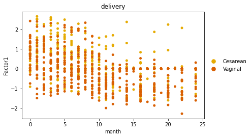
sc.pl.scatter(adata, x="month", y="Factor1", color="delivery",
              palette=sns.color_palette(cols4delivery.values()), size=100)
... storing 'group' as categorical
... storing 'delivery' as categorical
... storing 'diet' as categorical
... storing 'sex' as categorical
... storing 'Taxon' as categorical
... storing 'kingdom' as categorical
... storing 'phylum' as categorical
... storing 'class' as categorical
... storing 'order' as categorical
... storing 'family' as categorical
... storing 'genus' as categorical
... storing 'species' as categorical
[14]:
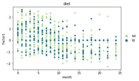
sc.pl.scatter(adata, x="month", y="Factor1", color="diet",
              palette=sns.color_palette(cols4diet.values()), size=100)
Downstream analysis#
For downstream analysis we can either use R (package MOFA2) or the Python package mofax. Here we will proceed in Python and first load the pre-trained model generated by the above steps.
[15]:
import mofax
[16]:
m = mofax.mofa_model(f"models/mefisto_microbiome.hdf5")
m
[16]:
MOFA+ model: mefisto microbiome
Samples (cells): 1032
Features: 969
Groups: C001 (24), C002 (24), C004 (24), C005 (24), C007 (24), C008 (24), C009 (24), C010 (24), C011 (24), C012 (24), C014 (24), C016 (24), C017 (24), C018 (24), C020 (24), C021 (24), C022 (24), C023 (24), C024 (24), C025 (24), C027 (24), C030 (24), C031 (24), C032 (24), C033 (24), C034 (24), C035 (24), C036 (24), C037 (24), C038 (24), C041 (24), C042 (24), C043 (24), C044 (24), C045 (24), C046 (24), C047 (24), C049 (24), C052 (24), C053 (24), C055 (24), C056 (24), C057 (24)
Views: data (969)
Factors: 2
Expectations: Sigma, W, Z

MEFISTO:
Covariates available: month
Variance decomposition and factor correlation#
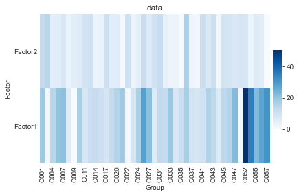
To obtain a first overview of the factors we can take a look at the variance that a factor explains in each child.
[17]:
mofax.plot_r2(m, cmap="Blues")
[17]:
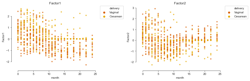
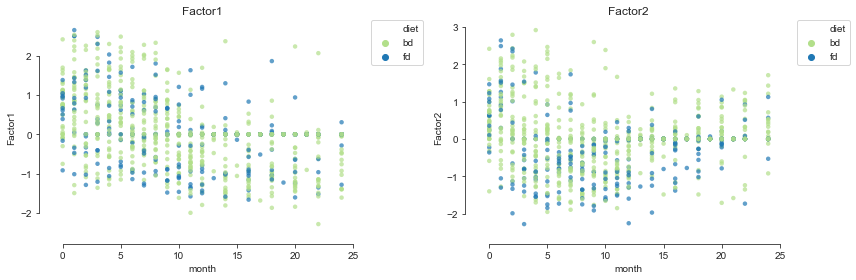
Factors versus month of life#
We can also plot the inferred factors against the months of life and colour them by the metadata of the samples taking advantage of a plotting function in mofax.
Using the first two factors, we can project the samples into a 2-dimensional space.
[18]:
mofax.plot_factors(m, x="month", y=[0, 1],
                   color="delivery", palette=cols4delivery, alpha=.7);
[19]:
mofax.plot_factors(m, x="month", y=[0, 1],
                   color="diet", palette=cols4diet, alpha=.7);
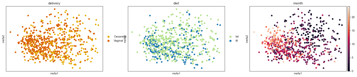
Scatterplot#
We can also look at the factor values on the sample level. Here each dot correspond to one time-point-child combination.
[20]:
mu.pl.mofa(adata, color=["delivery", "diet", "month"])
Factor weights#
Next we have a look at the microbial species associated with the factors, focusing on Factor 1. For this we have a look at the weights of the factor.
Individual species#
Let’s first have a look at the top positive and top negative species on factor 1. We find top negative weights for species of the genera Bacteroides and Faecalibacterium, meaning that their abundance varies in line with the negative of Factor 1, increasing over the first year of life and with higher abundance in vaginally delivered children.
[21]:
m.get_weights(factors="Factor1", df=True).join(m.features_metadata).sort_values("Factor1").head()
[21]:
| Factor1 | view | Confidence | Taxon | class | family | genus | kingdom | order | phylum | species | |
|---|---|---|---|---|---|---|---|---|---|---|---|
| c4f9ef34bd2919511069f409c25de6f1 | -2.010341 | data | 0.999160 | k__Bacteria; p__Bacteroidetes; c__Bacteroidia;... | c__Bacteroidia | f__Bacteroidaceae | g__Bacteroides | k__Bacteria | o__Bacteroidales | p__Bacteroidetes | s__ |
| 010f0ac2691bc0be12d0633d4b5d2cc4 | -1.978174 | data | 0.999978 | k__Bacteria; p__Firmicutes; c__Clostridia; o__... | c__Clostridia | f__Ruminococcaceae | g__Faecalibacterium | k__Bacteria | o__Clostridiales | p__Firmicutes | s__prausnitzii |
| ac5402de1ddf427ab8d2b0a8a0a44f19 | -1.877653 | data | 0.999770 | k__Bacteria; p__Bacteroidetes; c__Bacteroidia;... | c__Bacteroidia | f__Bacteroidaceae | g__Bacteroides | k__Bacteria | o__Bacteroidales | p__Bacteroidetes | s__ |
| 8937656c16c20701c107e715bad86732 | -1.603405 | data | 0.758990 | k__Bacteria; p__Firmicutes; c__Clostridia; o__... | c__Clostridia | f__Lachnospiraceae | g__Roseburia | k__Bacteria | o__Clostridiales | p__Firmicutes | s__faecis |
| 2a99ec1157a90661db7ff643b82f1914 | -1.569408 | data | 0.997669 | k__Bacteria; p__Bacteroidetes; c__Bacteroidia;... | c__Bacteroidia | f__Bacteroidaceae | g__Bacteroides | k__Bacteria | o__Bacteroidales | p__Bacteroidetes | s__fragilis |
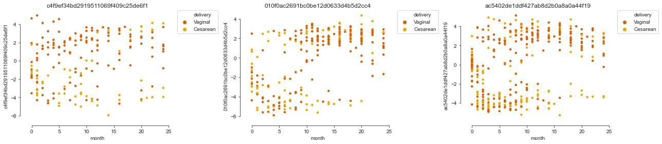
We can also take a look at the data for the top features on the factor:
[22]:
mofax.plot_factors(m, x="month", y=m.get_top_features(factors="Factor1", n_features=3), color="delivery", palette=cols4delivery);
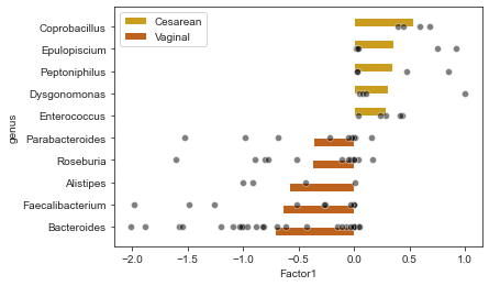
Aggregation to genus level#
We now aggregate the weights on the genus level.
[23]:
df_weights = (
    m.get_weights(df=True, factors="Factor1")
     .join(m.features_metadata)
     .query("genus != 'g__'")
)

df_weights.genus = df_weights.genus.str.replace('g__', '').str.replace('\\[', '').str.replace('\\]', '')

# summarize by mean weights across all species in the genus
# and filter to top 10 positive and negative ones
df_top = (
    df_weights
    .groupby("genus")
    .agg(mean_weight=("Factor1", "mean"),
         n_spec=("Factor1", "size"))
    .query("n_spec > 2")
    .reset_index()
    .assign(type=lambda x: np.where(x["mean_weight"] > 0, "Cesarean", "Vaginal"),
            mean_weight_abs=lambda x: np.abs(x["mean_weight"]))
    .groupby("type")
    .apply(lambda x: x.nlargest(5, "mean_weight_abs"))
    .sort_values("mean_weight", ascending=False)
    .reset_index(drop=1)
)
[24]:
df_top
[24]:
| genus | mean_weight | n_spec | type | mean_weight_abs | |
|---|---|---|---|---|---|
| 0 | Coprobacillus | 0.529192 | 4 | Cesarean | 0.529192 |
| 1 | Epulopiscium | 0.350463 | 5 | Cesarean | 0.350463 |
| 2 | Peptoniphilus | 0.342736 | 4 | Cesarean | 0.342736 |
| 3 | Dysgonomonas | 0.309555 | 4 | Cesarean | 0.309555 |
| 4 | Enterococcus | 0.281913 | 5 | Cesarean | 0.281913 |
| 5 | Parabacteroides | -0.369146 | 9 | Vaginal | 0.369146 |
| 6 | Roseburia | -0.381634 | 12 | Vaginal | 0.381634 |
| 7 | Alistipes | -0.583242 | 4 | Vaginal | 0.583242 |
| 8 | Faecalibacterium | -0.643833 | 9 | Vaginal | 0.643833 |
| 9 | Bacteroides | -0.712832 | 25 | Vaginal | 0.712832 |
[25]:
ax = sns.barplot(data=df_top, x="mean_weight", y="genus", hue="type", palette=cols4delivery)
sns.scatterplot(data=df_weights[df_weights.genus.isin(df_top.genus)].set_index("genus").loc[df_top.genus,:].reset_index(),
                x="Factor1", y="genus", color="black", alpha=.5, ax=ax, zorder=10);
More details are discussed in the original R and Python notebooks.