Identifying temporal variation in EvoDevo data with MEFISTO
Contents
Identifying temporal variation in EvoDevo data with MEFISTO#
This notebook demonstrates how temporal (or spatial) covariates can be used for multimodal data integration to learn smooth latent factors while benefiting from the multimodal MuData objects from muon.
Please find more information about this method — MEFISTO — on its website and in the preprint by Britta Velten et al.
[1]:
import numpy as np
import pandas as pd
import scanpy as sc

import muon as mu
[2]:
# Set the working directory to the root of the repository
import os
os.chdir("../")
Load data#
First we will load the evodevo data containing normalized gene expression data for 5 species (groups) and 5 organs (views) as well as the developmental time information for each sample. The data can be downloaded from here.
[3]:
datadir = "data/evodevo"
[4]:
data = pd.read_csv(f"{datadir}/evodevo.csv", sep=",", index_col=0)
data
/usr/local/lib/python3.8/site-packages/numpy/lib/arraysetops.py:583: FutureWarning: elementwise comparison failed; returning scalar instead, but in the future will perform elementwise comparison
  mask |= (ar1 == a)
[4]:
| group | view | sample | feature | value | time | |
|---|---|---|---|---|---|---|
| 1 | Human | Brain | 10wpc_Human | ENSG00000000457_Brain | 8.573918 | 7 |
| 2 | Human | Brain | 10wpc_Human | ENSG00000001084_Brain | 8.875957 | 7 |
| 3 | Human | Brain | 10wpc_Human | ENSG00000001167_Brain | 11.265237 | 7 |
| 4 | Human | Brain | 10wpc_Human | ENSG00000001461_Brain | 7.374965 | 7 |
| 5 | Human | Brain | 10wpc_Human | ENSG00000001561_Brain | 7.311018 | 7 |
| ... | ... | ... | ... | ... | ... | ... |
| 3193836 | Human | Testis | youngMidAge_Human | ENSG00000271503_Testis | 1.178014 | 21 |
| 3193837 | Human | Testis | youngMidAge_Human | ENSG00000271601_Testis | 1.178014 | 21 |
| 3193838 | Human | Testis | youngMidAge_Human | ENSG00000272442_Testis | 4.476201 | 21 |
| 3193839 | Human | Testis | youngMidAge_Human | ENSG00000272886_Testis | 1.178014 | 21 |
| 3193840 | Human | Testis | youngMidAge_Human | ENSG00000273079_Testis | 8.311393 | 21 |
3193840 rows × 6 columns
First, we create a collection of AnnData objects from this dataframe, one for each organ.
For instance, here’s the data for the 'Brain' view:
[5]:
brain = data[data.view == 'Brain'].pivot(index='sample', columns='feature', values='value')
brain
[5]:
| feature | ENSG00000000457_Brain | ENSG00000001084_Brain | ENSG00000001167_Brain | ENSG00000001461_Brain | ENSG00000001561_Brain | ENSG00000001617_Brain | ENSG00000001629_Brain | ENSG00000001631_Brain | ENSG00000002549_Brain | ENSG00000002745_Brain | ... | ENSG00000267909_Brain | ENSG00000268104_Brain | ENSG00000269058_Brain | ENSG00000270885_Brain | ENSG00000271092_Brain | ENSG00000271503_Brain | ENSG00000271601_Brain | ENSG00000272442_Brain | ENSG00000272886_Brain | ENSG00000273079_Brain |
|---|---|---|---|---|---|---|---|---|---|---|---|---|---|---|---|---|---|---|---|---|---|
| sample | |||||||||||||||||||||
| 10wpc_Human | 8.573918 | 8.875957 | 11.265237 | 7.374965 | 7.311018 | 9.959839 | 10.542619 | 9.692082 | 9.180280 | 4.281878 | ... | 7.221091 | 1.178014 | 1.178014 | 1.178014 | 1.178014 | 1.178014 | 1.178014 | 1.178014 | 1.178014 | 11.74615 |
| 11wpc_Human | 8.439675 | 8.737682 | 10.855314 | 8.066544 | 7.354726 | 10.431113 | 10.308780 | 9.242115 | 9.350255 | 3.363064 | ... | 7.116983 | 1.178014 | 1.178014 | 1.178014 | 1.178014 | 1.178014 | 1.178014 | 1.421384 | 1.178014 | 11.28160 |
| 12wpc_Human | 8.399178 | 8.916387 | 12.555510 | 9.253555 | 8.763702 | 9.946536 | 11.530929 | 10.033949 | 9.278142 | 4.322361 | ... | 4.000716 | 1.178014 | 1.178014 | 1.178014 | 1.178014 | 1.178014 | 1.178014 | 2.664630 | 1.178014 | 13.97646 |
| 13wpc_Human | 8.637347 | 8.831740 | 10.916489 | 9.190959 | 8.158240 | 10.279600 | 11.287268 | 9.510370 | 9.033614 | 4.784136 | ... | 5.635512 | 1.178014 | 1.481758 | 1.178014 | 1.178014 | 1.178014 | 1.178014 | 1.776655 | 1.178014 | 12.47349 |
| 16wpc_Human | 8.525125 | 8.575862 | 11.271736 | 8.177629 | 7.857303 | 10.363036 | 11.402954 | 9.523244 | 8.833177 | 2.785827 | ... | 6.119527 | 1.178014 | 1.178014 | 1.178014 | 1.178014 | 1.178014 | 1.178014 | 2.413222 | 1.178014 | 13.73805 |
| ... | ... | ... | ... | ... | ... | ... | ... | ... | ... | ... | ... | ... | ... | ... | ... | ... | ... | ... | ... | ... | ... |
| senior_Human | 8.437410 | 9.898419 | 8.216911 | 11.504150 | 9.958047 | 6.857990 | 9.623469 | 9.205518 | 9.884420 | 4.484028 | ... | 3.862928 | 1.178014 | 2.254255 | 1.178014 | 1.178014 | 1.178014 | 1.178014 | 2.581292 | 1.178014 | 11.67438 |
| teenager_Human | 8.429526 | 9.949921 | 8.637132 | 11.680144 | 10.211024 | 6.452668 | 10.214713 | 9.604091 | 9.903370 | 5.265158 | ... | 3.162686 | 1.178014 | 1.178014 | 1.178014 | 1.453269 | 1.178014 | 1.178014 | 3.016177 | 1.178014 | 12.54986 |
| toddler_Human | 8.333979 | 10.027861 | 8.693345 | 11.691258 | 9.731870 | 7.191969 | 10.286671 | 8.958592 | 10.120605 | 5.322412 | ... | 5.152286 | 1.178014 | 1.648489 | 1.178014 | 1.178014 | 1.178014 | 1.178014 | 3.201100 | 1.178014 | 12.81460 |
| youngAdult_Human | 8.601354 | 10.237539 | 9.176577 | 12.092567 | 10.388409 | 6.998035 | 10.577031 | 9.812306 | 9.798473 | 5.154397 | ... | 4.365919 | 1.178014 | 1.178014 | 1.178014 | 1.178014 | 1.178014 | 1.178014 | 3.330907 | 1.178014 | 12.69678 |
| youngMidAge_Human | 8.378206 | 9.924419 | 9.128045 | 11.684351 | 10.253423 | 6.914197 | 10.260315 | 9.917214 | 9.823436 | 4.722714 | ... | 4.218114 | 1.178014 | 3.464638 | 1.178014 | 1.737065 | 1.178014 | 1.178014 | 3.069621 | 1.178014 | 12.59430 |
83 rows × 7696 columns
[6]:
views = data.view.unique()
data_list = [data[data.view == m].pivot(index='sample', columns='feature', values='value') for m in views]
mods = {views[m]:sc.AnnData(data_list[m]) for m in range(len(views))}
mods
[6]:
{'Brain': AnnData object with n_obs × n_vars = 83 × 7696,
 'Cerebellum': AnnData object with n_obs × n_vars = 83 × 7696,
 'Heart': AnnData object with n_obs × n_vars = 83 × 7696,
 'Liver': AnnData object with n_obs × n_vars = 83 × 7696,
 'Testis': AnnData object with n_obs × n_vars = 83 × 7696}
In addition, we keep the meta data for each sample, containing the developmental time points.
[7]:
obs = (
    data[['sample', 'time', 'group']]
        .drop_duplicates()
        .rename(columns = {'group' : 'species'})
        .set_index('sample')
)
obs
[7]:
| time | species | |
|---|---|---|
| sample | ||
| 10wpc_Human | 7 | Human |
| 11wpc_Human | 8 | Human |
| 12wpc_Human | 9 | Human |
| 13wpc_Human | 10 | Human |
| 16wpc_Human | 11 | Human |
| ... | ... | ... |
| senior_Human | 23 | Human |
| teenager_Human | 19 | Human |
| toddler_Human | 17 | Human |
| youngAdult_Human | 20 | Human |
| youngMidAge_Human | 21 | Human |
83 rows × 2 columns
We now create a multimodal MuData object:
[8]:
mdata = mu.MuData(mods)
mdata.obs = mdata.obs.join(obs)
This contains both the gene expression data,
[9]:
print(mdata)
mdata["Brain"]
MuData object with n_obs × n_vars = 83 × 38480
  obs:  'time', 'species'
  5 modalities
    Brain:      83 x 7696
    Cerebellum: 83 x 7696
    Heart:      83 x 7696
    Liver:      83 x 7696
    Testis:     83 x 7696
[9]:
AnnData object with n_obs × n_vars = 83 × 7696
as well as the sample-level information given by the developmental time points, which are not yet matched for different species.
[10]:
mdata.obs
[10]:
| time | species | |
|---|---|---|
| sample | ||
| 10wpc_Human | 7 | Human |
| 11wpc_Human | 8 | Human |
| 12wpc_Human | 9 | Human |
| 13wpc_Human | 10 | Human |
| 16wpc_Human | 11 | Human |
| ... | ... | ... |
| senior_Human | 23 | Human |
| teenager_Human | 19 | Human |
| toddler_Human | 17 | Human |
| youngAdult_Human | 20 | Human |
| youngMidAge_Human | 21 | Human |
83 rows × 2 columns
Integrate data#
MEFISTO can be run on a MuData object with mu.tl.mofa by specifying which variable (covariate) should be treated as time.
To incorporate the time information, we specify which metadata column to use as a covariate for MEFISTO —
'time'.We also specify
'species'to be used as groups.In addition, we tell the model that we want to learn an alignment of the time points from different species by setting
smooth_warping=Trueand using'Mouse'as reference.Using the underlying Gaussian process for each factor we can interpolate to unseen time points. This is enabled by providing
new_values, which correspond to the covariate, i.e. time.
For illustration, we only use a small number of training iterations.
[11]:
mu.tl.mofa(mdata, n_factors=5,
           groups_label="species",
           smooth_covariate='time', smooth_warping=True,
           smooth_kwargs={"warping_ref": "Mouse", "new_values": list(range(1, 15))},
           outfile="models/mefisto_evodevo.hdf5",
           n_iterations=25)
        #########################################################
        ###           __  __  ____  ______                    ###
        ###          |  \/  |/ __ \|  ____/\    _             ###
        ###          | \  / | |  | | |__ /  \ _| |_           ###
        ###          | |\/| | |  | |  __/ /\ \_   _|          ###
        ###          | |  | | |__| | | / ____ \|_|            ###
        ###          |_|  |_|\____/|_|/_/    \_\              ###
        ###                                                   ###
        #########################################################


Loaded view='Brain' group='Human' with N=23 samples and D=7696 features...
Loaded view='Brain' group='Mouse' with N=14 samples and D=7696 features...
Loaded view='Brain' group='Opossum' with N=15 samples and D=7696 features...
Loaded view='Brain' group='Rabbit' with N=15 samples and D=7696 features...
Loaded view='Brain' group='Rat' with N=16 samples and D=7696 features...
Loaded view='Cerebellum' group='Human' with N=23 samples and D=7696 features...
Loaded view='Cerebellum' group='Mouse' with N=14 samples and D=7696 features...
Loaded view='Cerebellum' group='Opossum' with N=15 samples and D=7696 features...
Loaded view='Cerebellum' group='Rabbit' with N=15 samples and D=7696 features...
Loaded view='Cerebellum' group='Rat' with N=16 samples and D=7696 features...
Loaded view='Heart' group='Human' with N=23 samples and D=7696 features...
Loaded view='Heart' group='Mouse' with N=14 samples and D=7696 features...
Loaded view='Heart' group='Opossum' with N=15 samples and D=7696 features...
Loaded view='Heart' group='Rabbit' with N=15 samples and D=7696 features...
Loaded view='Heart' group='Rat' with N=16 samples and D=7696 features...
Loaded view='Liver' group='Human' with N=23 samples and D=7696 features...
Loaded view='Liver' group='Mouse' with N=14 samples and D=7696 features...
Loaded view='Liver' group='Opossum' with N=15 samples and D=7696 features...
Loaded view='Liver' group='Rabbit' with N=15 samples and D=7696 features...
Loaded view='Liver' group='Rat' with N=16 samples and D=7696 features...
Loaded view='Testis' group='Human' with N=23 samples and D=7696 features...
Loaded view='Testis' group='Mouse' with N=14 samples and D=7696 features...
Loaded view='Testis' group='Opossum' with N=15 samples and D=7696 features...
Loaded view='Testis' group='Rabbit' with N=15 samples and D=7696 features...
Loaded view='Testis' group='Rat' with N=16 samples and D=7696 features...


Model options:
- Automatic Relevance Determination prior on the factors: True
- Automatic Relevance Determination prior on the weights: True
- Spike-and-slab prior on the factors: False
- Spike-and-slab prior on the weights: True
Likelihoods:
- View 0 (Brain): gaussian
- View 1 (Cerebellum): gaussian
- View 2 (Heart): gaussian
- View 3 (Liver): gaussian
- View 4 (Testis): gaussian


Loaded 1 covariate(s) for each sample...


Smooth covariate framework is activated. This is not compatible with ARD prior on factors. Setting ard_factors to False...

##
## Warping set to True: aligning the covariates across groups
##


######################################
## Training the model with seed 1 ##
######################################


Importing the dtw module. When using in academic works please cite:
  T. Giorgino. Computing and Visualizing Dynamic Time Warping Alignments in R: The dtw Package.
  J. Stat. Soft., doi:10.18637/jss.v031.i07.

Covariates were aligned between groups.
Optimising sigma node...


#######################
## Training finished ##
#######################


Warning: Output file models/mefisto_evodevo.hdf5 already exists, it will be replaced
Saving model in models/mefisto_evodevo.hdf5...
Saved MOFA embeddings in .obsm['X_mofa'] slot and their loadings in .varm['LFs'].
Visualization in the factor space#
[14]:
import seaborn as sns
palette = sns.color_palette("Set2")
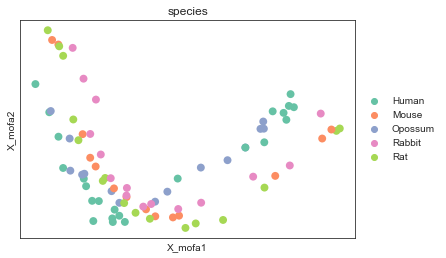
Let’s take a look at the decomposition learnt by the model.
[15]:
mu.pl.mofa(mdata, color="species", palette=palette, size = 250)
... storing 'species' as categorical
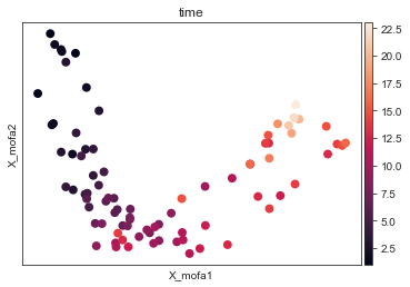
[16]:
mu.pl.mofa(mdata, color="time", size = 250)
... storing 'species' as categorical
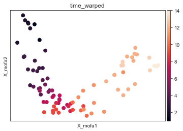
[17]:
mu.pl.mofa(mdata, color="time_warped", size = 250)
... storing 'species' as categorical
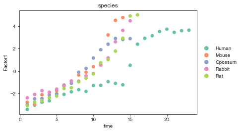
Latent factors versus common developmental time#
We can plot the latent processes along the inferred common developmental time.
[18]:
mdata.obs["Factor1"] = mdata.obsm["X_mofa"][:,0]
Before alignment:
[19]:
import seaborn as sns
sc.pl.scatter(mdata, x="time", y="Factor1", color="species",
              palette=palette, size=200)
... storing 'species' as categorical
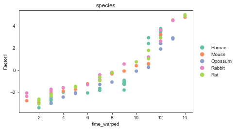
After alignment:
[20]:
sc.pl.scatter(mdata, x="time_warped", y="Factor1", color="species",
              palette=palette, size=200)
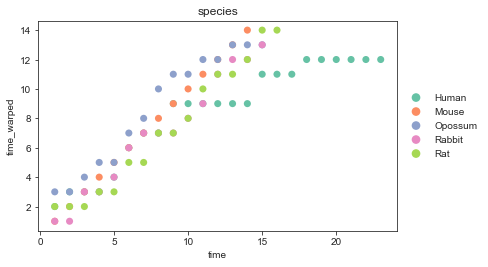
Alignment#
We can also take a look at the learnt alignemnt.
[21]:
sc.pl.scatter(mdata, x="time", y="time_warped", color="species",
              palette=palette, size=200)
Further analyses#
Additionally we can take a look at the smoothness and sharedness of the factors, interpolate the factors or cluster the species based on the learnt group kernel of each latent factor.
For that, we will use the mofax library that provides convenient loaders and plotting functions.
[22]:
import mofax
model = mofax.mofa_model("models/mefisto_evodevo.hdf5")
model
[22]:
MOFA+ model: mefisto evodevo
Samples (cells): 83
Features: 38480
Groups: Human (23), Mouse (14), Opossum (15), Rabbit (15), Rat (16)
Views: Brain (7696), Cerebellum (7696), Heart (7696), Liver (7696), Testis (7696)
Factors: 5
Expectations: Sigma, W, Z

MEFISTO:
Covariates available: time
Interpolated factors for 14 new values
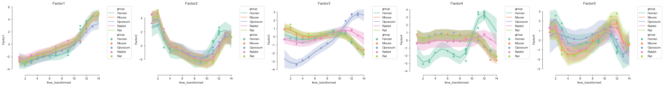
Interpolation#
Using the underlying Gaussian process for each factor we can interpolate to unseen time points for species that are missing data in these time points or intermediate time points.
[23]:
mofax.plot_interpolated_factors(model, factors=range(model.nfactors),
                                ncols=5, size=70);
Smoothness and sharedness of factors#
In addition to the factor values and the alignment the model also inferred an underlying Gaussian process that generated these values. By looking into it we can extract information on the smoothness of each factor, i.e. how smoothly it varies along developmental time, as well as the sharedness of each factor, i.e. how much the species (groups) show the same underlying developmental pattern and how the shape of their developmental trajectory related to a given developmental module (Factor) clusters between species.
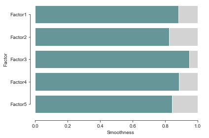
The scale parameters of the Gaussian process capture the smoothness of the model. We will visualize them with bar plots where more colour means more smoothness:
[24]:
mofax.plot_smoothness(model);
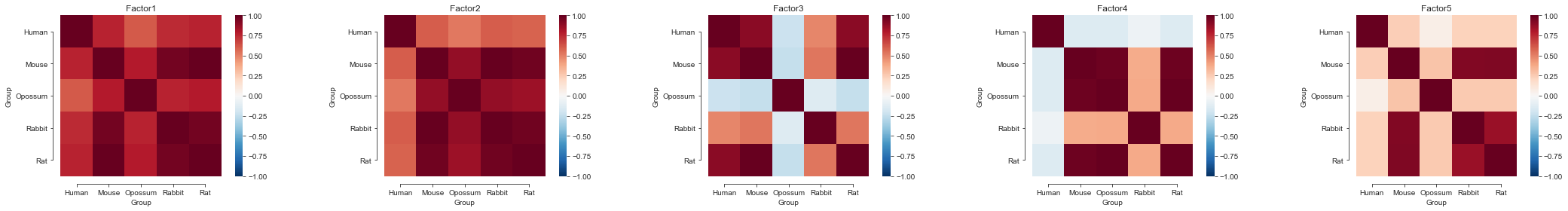
The group kernel of the Gaussian process can give us insights into the extent to which a temporal pattern is shared across species for the developmental module captured by each process:
[27]:
mofax.plot_group_kernel(model, ncols=5);
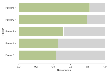
We can also plot sharedness as a feature for each factor (fully coloured bar means fully shared):
[29]:
mofax.plot_sharedness(model);