MEFISTO application to spatial transcriptomics
Contents
MEFISTO application to spatial transcriptomics#
This notebook demonstrates how MEFISTO can be applied to spatial transcriptomics using its interface for muon.
R vignette for this application is available here.
We use the "Mouse Brain Serial Section 1 (Sagittal-Anterior)" dataset provided by 10X Genomics. The following files are used in this tutorial:
Feature / cell matrix HDF5 (filtered) (
filtered_feature_bc_matrix.h5),Spatial imaging data (
spatial.tar.gz, has to be unarchived).
[1]:
import numpy as np
import pandas as pd
import scanpy as sc

import matplotlib.pyplot as plt
import seaborn as sns

import muon as mu
[2]:
# Set the working directory to the root of the repository
import os
os.chdir("../")
Load data#
In this notebook, we put the files mentioned above into the data/ST/ directory.
[3]:
datadir = "data/ST/"
[4]:
adata = sc.read_visium(datadir)
Variable names are not unique. To make them unique, call `.var_names_make_unique`.
Variable names are not unique. To make them unique, call `.var_names_make_unique`.
[5]:
adata
[5]:
AnnData object with n_obs × n_vars = 2695 × 32285
    obs: 'in_tissue', 'array_row', 'array_col'
    var: 'gene_ids', 'feature_types', 'genome'
    uns: 'spatial'
    obsm: 'spatial'
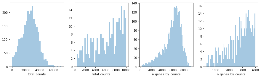
QC and preprocessing#
We will follow scanpy’s spatial tutorial for the steps below.
[6]:
adata.var["mt"] = adata.var_names.str.startswith("mt-")
sc.pp.calculate_qc_metrics(adata, qc_vars=["mt"], inplace=True)
[7]:
fig, axs = plt.subplots(1, 4, figsize=(15, 4))
sns.distplot(adata.obs["total_counts"], kde=False, ax=axs[0])
sns.distplot(adata.obs["total_counts"][adata.obs["total_counts"] < 10000], kde=False, bins=40, ax=axs[1])
sns.distplot(adata.obs["n_genes_by_counts"], kde=False, bins=60, ax=axs[2])
sns.distplot(adata.obs["n_genes_by_counts"][adata.obs["n_genes_by_counts"] < 4000], kde=False, bins=60, ax=axs[3])
[7]:
<AxesSubplot:xlabel='n_genes_by_counts'>
[8]:
mu.pp.filter_obs(adata, 'total_counts', lambda x: x < 50000)
mu.pp.filter_obs(adata, 'pct_counts_mt', lambda x: x < 20)
mu.pp.filter_var(adata, 'n_cells_by_counts', lambda x: x > 10)
[9]:
sc.pp.normalize_total(adata, inplace=True)
sc.pp.log1p(adata)
sc.pp.highly_variable_genes(adata, flavor="seurat", n_top_genes=2000)
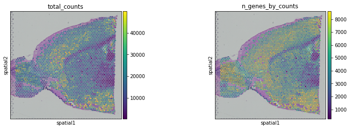
[10]:
sc.pl.spatial(adata, img_key="hires", color=["total_counts", "n_genes_by_counts"])
... storing 'feature_types' as categorical
... storing 'genome' as categorical
We will now add spatial covariates to the .obs slot so that we can refer to them easily later:
[11]:
adata.obs = pd.concat([adata.obs,
                       pd.DataFrame(adata.obsm["spatial"], columns=["imagerow", "imagecol"], index=adata.obs_names),
                      ], axis=1)
Train a MEFISTO model#
[12]:
# We use 1000 inducing points to learn spatial covariance patterns
n_inducing = 1000
[13]:
mu.tl.mofa(adata, n_factors=4,
           smooth_covariate=["imagerow", "imagecol"],
           smooth_kwargs={
               "sparseGP": True, "frac_inducing": n_inducing/adata.n_obs,
               "start_opt": 10, "opt_freq": 10,
           },
           outfile="models/mefisto_ST.hdf5",
           use_float32=True, seed=2021,
           quiet=False)
Variable names are not unique. To make them unique, call `.var_names_make_unique`.
        #########################################################
        ###           __  __  ____  ______                    ###
        ###          |  \/  |/ __ \|  ____/\    _             ###
        ###          | \  / | |  | | |__ /  \ _| |_           ###
        ###          | |\/| | |  | |  __/ /\ \_   _|          ###
        ###          | |  | | |__| | | / ____ \|_|            ###
        ###          |_|  |_|\____/|_|/_/    \_\              ###
        ###                                                   ###
        #########################################################


use_float32 set to True: replacing float64 arrays by float32 arrays to speed up computations...

Loaded view='rna' group='group1' with N=2448 samples and D=2000 features...


Model options:
- Automatic Relevance Determination prior on the factors: True
- Automatic Relevance Determination prior on the weights: True
- Spike-and-slab prior on the factors: False
- Spike-and-slab prior on the weights: True
Likelihoods:
- View 0 (rna): gaussian


Loaded 2 covariate(s) for each sample...


Smooth covariate framework is activated. This is not compatible with ARD prior on factors. Setting ard_factors to False...

##
## sparseGP set to True: using sparse Gaussian Process to speed up the training procedure
##


######################################
## Training the model with seed 2021 ##
######################################


ELBO before training: -18465131.15

Iteration 1: time=2.13, ELBO=-1458115.86, deltaELBO=17007015.287 (92.10340913%), Factors=4
Iteration 2: time=2.34, ELBO=-1351293.76, deltaELBO=106822.096 (0.57850711%), Factors=4
Iteration 3: time=2.20, ELBO=-1338817.69, deltaELBO=12476.078 (0.06756561%), Factors=4
Iteration 4: time=2.11, ELBO=-1334998.85, deltaELBO=3818.836 (0.02068133%), Factors=4
Iteration 5: time=2.18, ELBO=-1331967.83, deltaELBO=3031.026 (0.01641486%), Factors=4
Iteration 6: time=2.12, ELBO=-1329438.70, deltaELBO=2529.124 (0.01369676%), Factors=4
Iteration 7: time=2.13, ELBO=-1327417.88, deltaELBO=2020.818 (0.01094397%), Factors=4
Iteration 8: time=2.14, ELBO=-1325906.92, deltaELBO=1510.962 (0.00818278%), Factors=4
Iteration 9: time=2.16, ELBO=-1324828.37, deltaELBO=1078.550 (0.00584101%), Factors=4
Optimising sigma node...
Iteration 10: time=420.53, ELBO=-1278645.02, deltaELBO=46183.350 (0.25011114%), Factors=4
Iteration 11: time=12.73, ELBO=-1345144.36, deltaELBO=-66499.341 (0.36013468%), Factors=4
Warning, lower bound is decreasing...
Iteration 12: time=12.74, ELBO=-1338754.04, deltaELBO=6390.321 (0.03460750%), Factors=4
Iteration 13: time=12.94, ELBO=-1335177.18, deltaELBO=3576.864 (0.01937091%), Factors=4
Iteration 14: time=12.74, ELBO=-1332578.48, deltaELBO=2598.698 (0.01407354%), Factors=4
Iteration 15: time=12.57, ELBO=-1330587.59, deltaELBO=1990.894 (0.01078191%), Factors=4
Iteration 16: time=12.95, ELBO=-1329018.00, deltaELBO=1569.581 (0.00850024%), Factors=4
Iteration 17: time=12.65, ELBO=-1327749.26, deltaELBO=1268.741 (0.00687101%), Factors=4
Iteration 18: time=12.83, ELBO=-1326705.46, deltaELBO=1043.804 (0.00565284%), Factors=4
Iteration 19: time=12.74, ELBO=-1325836.99, deltaELBO=868.467 (0.00470328%), Factors=4
Optimising sigma node...
Iteration 20: time=1496.66, ELBO=-1325009.56, deltaELBO=827.436 (0.00448107%), Factors=4
Iteration 21: time=1168.83, ELBO=-1324128.00, deltaELBO=881.557 (0.00477417%), Factors=4
Iteration 22: time=27.07, ELBO=-1323403.16, deltaELBO=724.839 (0.00392545%), Factors=4
Iteration 23: time=25.32, ELBO=-1322812.93, deltaELBO=590.232 (0.00319647%), Factors=4
Iteration 24: time=23.43, ELBO=-1322311.74, deltaELBO=501.187 (0.00271423%), Factors=4
Iteration 25: time=21.34, ELBO=-1321880.57, deltaELBO=431.167 (0.00233504%), Factors=4
Iteration 26: time=22.70, ELBO=-1321505.86, deltaELBO=374.716 (0.00202932%), Factors=4
Iteration 27: time=21.14, ELBO=-1321176.73, deltaELBO=329.132 (0.00178245%), Factors=4
Iteration 28: time=21.43, ELBO=-1320884.46, deltaELBO=292.264 (0.00158279%), Factors=4
Iteration 29: time=23.10, ELBO=-1320621.24, deltaELBO=263.223 (0.00142552%), Factors=4
Optimising sigma node...
Iteration 30: time=2804.62, ELBO=-1320368.84, deltaELBO=252.402 (0.00136691%), Factors=4
Iteration 31: time=21.70, ELBO=-1323444.47, deltaELBO=-3075.632 (0.01665643%), Factors=4
Warning, lower bound is decreasing...
Iteration 32: time=20.51, ELBO=-1323195.89, deltaELBO=248.575 (0.00134619%), Factors=4
Iteration 33: time=20.16, ELBO=-1322989.62, deltaELBO=206.278 (0.00111712%), Factors=4
Iteration 34: time=20.54, ELBO=-1322806.93, deltaELBO=182.687 (0.00098936%), Factors=4
Iteration 35: time=20.13, ELBO=-1322644.66, deltaELBO=162.271 (0.00087880%), Factors=4
Iteration 36: time=20.15, ELBO=-1322500.42, deltaELBO=144.238 (0.00078114%), Factors=4
Iteration 37: time=21.20, ELBO=-1322372.32, deltaELBO=128.097 (0.00069372%), Factors=4
Iteration 38: time=22.12, ELBO=-1322258.70, deltaELBO=113.627 (0.00061536%), Factors=4
Iteration 39: time=944.91, ELBO=-1322157.73, deltaELBO=100.965 (0.00054679%), Factors=4
Optimising sigma node...
Iteration 40: time=1357.02, ELBO=-1322066.72, deltaELBO=91.011 (0.00049288%), Factors=4
Iteration 41: time=12.95, ELBO=-1322113.39, deltaELBO=-46.673 (0.00025276%), Factors=4
Warning, lower bound is decreasing...

Converged!


#######################
## Training finished ##
#######################


Saving model in models/mefisto_ST.hdf5...
Saved MOFA embeddings in .obsm['X_mofa'] slot and their loadings in .varm['LFs'].
Downstream analyses#
For some of the functionality below we will also use mofax.
[14]:
import mofax
m = mofax.mofa_model("models/mefisto_ST.hdf5")
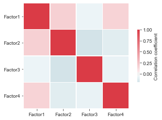
Factors correlation#
First, we can take a look whether our factor are uncorrelated.
[15]:
mofax.plot_factors_correlation(m);
Spatial factors#
We will then have a look at the spatial patterns that are captured by each factor.
[16]:
for i in range(4):
    adata.obs[f"Factor{i+1}"] = adata.obsm["X_mofa"][:,i]
[17]:
sc.pl.spatial(adata, img_key="hires", color=[f"Factor{i+1}" for i in range(4)])
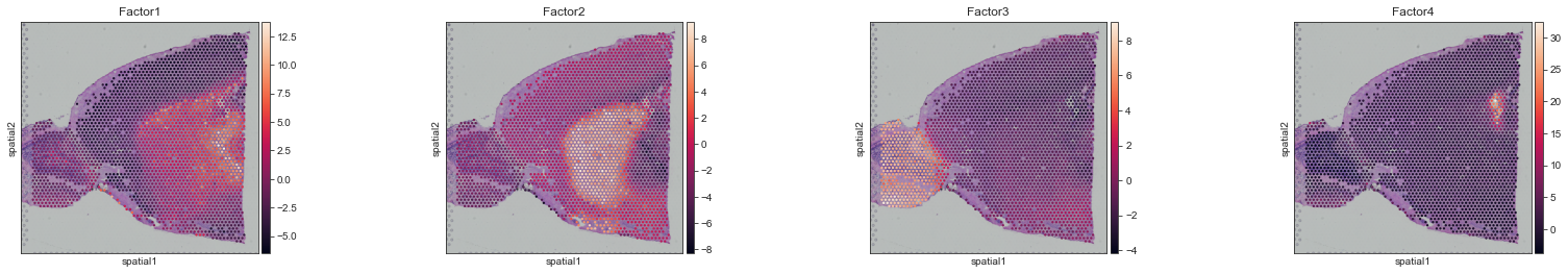
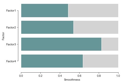
Smoothness of factors#
All of this factors seem to capture spatial patterns of variation that seems to vary smoothly along space to some extent. We can take a look at the smoothness score inferred by the model.
[18]:
mofax.plot_smoothness(m)
[18]:
<AxesSubplot:xlabel='Smoothness', ylabel='Factor'>
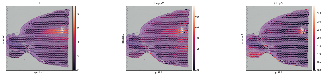
Weights#
We will take Factor4 as an example to show the spatial expression pattern for genes that have the highest weights for that factor.
[19]:
top_features_f4 = m.get_top_features(factors="Factor4", n_features=3)
top_features_f4
[19]:
array(['Ttr', 'Enpp2', 'Igfbp2'], dtype=object)
[20]:
sc.pl.spatial(adata, img_key="hires", color=top_features_f4)